
Executive Summary
Raw-water quality reports commonly provide mean, minimum and maximum values alongside a set of routine indicators. Yet the reliability of a drinking-water treatment plant depends less on the long-term average of any single parameter than on how contaminants vary over time, whether unfavorable conditions coincide, how long these conditions persist, and whether the treatment train can maintain finished-water quality throughout an event.
Two sources with the same annual mean turbidity may require very different coagulation controls, solids-separation capacity, filter redundancy, chemical inventories and emergency procedures. One source may be relatively stable throughout the year; another may be clear most of the time but experience a high-turbidity shock lasting hours or days after a storm. Reducing both to a single average erases some of the most important design information.
This article introduces a Design Raw-Water Quality Envelope: define the finished-water objectives and treatment barriers first; assemble a traceable dataset; identify seasonal, event-driven and long-term variation; examine relationships among key variables; define representative normal, validated upset and beyond-validated scenarios; and translate them into equipment constraints, operating windows, monitoring requirements and exceedance actions.
Two kinds of examples are used. The first is an ATLAS-constructed engineering calculation comparing two hypothetical sources that have the same mean turbidity but different temporal patterns. The second is the documented 2014 Toledo, Ohio, microcystin incident, using only event facts and figures from a US EPA report, not EPA photographs, charts or extended excerpts. The lesson is that a defensible design basis must address event recognition, adjustable treatment capability, finished-water verification, event duration and supply decisions outside the validated envelope, not concentration alone.
Editorial note | Data sources and rights. The analysis, engineering framework, illustrative calculations and all SVG figures were independently developed by ATLAS WTS. Toledo event data come from the US EPA Recommendations for Public Water Systems to Manage Cyanotoxins in Drinking Water (EPA 815-R-15-010). Only necessary facts are paraphrased and linked; no EPA imagery, layout or lengthy text has been reproduced. EPA cautions that individual files on its website may have different rights restrictions. WHO, AWWA and Water Research Foundation materials were used to cross-check methods; copyrighted graphics and prose were not copied.
01 | How Can Identical Averages Imply Very Different Treatment Plants?
Consider two hypothetical sources compared over 30 consecutive days using one representative daily turbidity reading.
Source A: 29 days at 10 NTU and one day at 310 NTU.
Source B: 30 days at 20 NTU.
Both have the same arithmetic mean:
Source A = (29 × 10 + 1 × 310) / 30 = 20 NTU
Source B = (30 × 20) / 30 = 20 NTU
However, they are not equivalent for process design.
Source B presents a relatively stable particle load. Coagulant feed, flocculation conditions, clarifier solids loading and filter run length can be maintained within a comparatively steady operating window. Seasonal and temperature effects still matter, but control focuses mainly on stability and efficiency.
Source A instead presents a short-duration shock-loading challenge. If the 310-NTU event coincides with changes in particle character, flow, low temperature or increased natural organic matter, coagulant demand, sludge production, filter loading and backwash frequency may shift rapidly. Even a one-day event can govern maximum metering-pump capacity, chemical reserves, sludge withdrawal capacity, filter redundancy and operator response time.
Equally important, a 310-NTU observation does not automatically require every unit at Source A to operate indefinitely at full flow under that condition. Engineers must ask:
- Does the event usually last 30 minutes, 6 hours, 24 hours or several days?
- Can intake flow be reduced during the event?
- Is raw-water balancing, clearwell storage, an alternative source or selective intake timing available?
- Are the particles readily removed by coagulation and settling, or dominated by difficult-to-settle fines?
- Does high turbidity coincide with DOC, pathogen hazards, agricultural runoff or other contaminants?
- Can the plant temporarily suspend or reduce intake when validated treatment capacity is exceeded?
A mean describes the general level over a period; it cannot, by itself, define treatment capability.
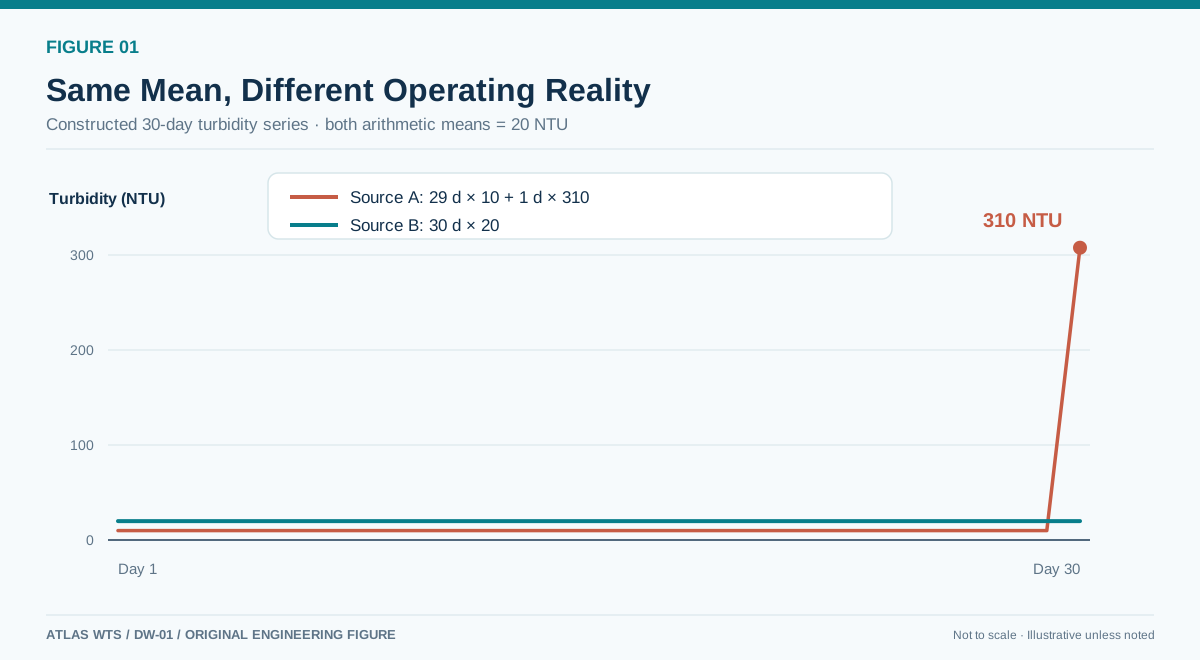
Figure 1 | Same mean, different temporal structure. These are illustrative ATLAS data, not measurements from real sources.
This is why a raw-water design basis must extend beyond the familiar mean/minimum/maximum table. Design-driving scenarios require a time dimension and an operational interpretation.
02 | Raw Water Is A Dynamic System, Not A Fixed Feed Composition
Engineering worksheets commonly describe raw water as a fixed list of turbidity, pH, alkalinity, hardness, TOC, temperature and target contaminant concentrations.
That is convenient for calculation, but risks implying that the parameters vary independently and each has a single representative value suitable for year-round operation. Real sources do not behave this way.
Seasonal change affects more than concentration
In rivers, lakes and reservoirs, seasons may change temperature, hydraulic residence time, algae, natural organic matter, storm runoff and water quality near different intake depths simultaneously.
Cold conditions alter reaction kinetics and floc development and may affect sustainable membrane flux and disinfection performance. Warm conditions may increase biological activity and complicate the management of blooms, taste-and-odor compounds and some organics.
Reservoirs may stratify thermally and mix seasonally. The same intake drawing from different depths or seasons may encounter different dissolved oxygen, iron, manganese, ammonia and organic-matter conditions.
A design basis must therefore establish not only how much of a contaminant is present on average, but under which temperature, pH, hydraulic and co-contaminant conditions it occurs.
Short events arise from different mechanisms
Intense rainfall can increase runoff, erosion and suspended solids. Drought can alter dilution, salinity or contaminant concentrations. Blooms may introduce algal cells, taste-and-odor compounds and cyanotoxins. An upstream accident can create a short contaminant pulse unrelated to seasonal processes.
These should not all be treated as one generic “maximum raw-water quality.”
Storm turbidity primarily challenges solids loading, coagulation flexibility, sludge removal and filtration. A toxin event requires differentiation between intracellular and dissolved constituents and verification of cell-removal, adsorption or oxidation barriers. The two may demand entirely different monitoring and emergency responses.
Long-term shifts reduce the representativeness of historical datasets
Land use, upstream discharges, agriculture, urbanization, reservoir operations and climate conditions can change the underlying source-water distribution.
A complete survey from ten years ago is not automatically more relevant than a recent, well-designed monitoring campaign. Record length matters, but so does the extent to which those records still represent future intake conditions.
For long-life infrastructure, distinguish:
- 01 historically observed conditions;
- 02 evidence-supported changes that may occur during the plant’s design life;
- 03 uncertainty not yet quantifiable, to be managed through monitoring, allowances and scalable design.
The third category should not be converted casually into a superficially precise safety factor.
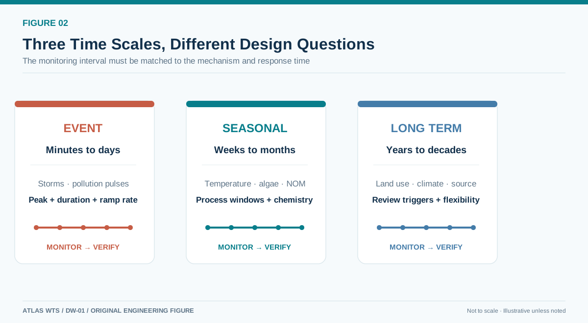
Figure 2 | Short events, seasonal cycles and long-term trends occur at different time scales, and therefore call for different monitoring and design responses.
The current WHO Guidelines for Drinking-water Quality continues to promote a preventive, catchment-to-consumer risk-management approach and Water Safety Plans. The envelope proposed here does not replace a WSP; it translates similar risk-management principles into engineering design inputs. WHO 2026 GDWQ
03 | Which Source-Water Parameters Actually Govern Treatment?
More measurements are not automatically better. A useful monitoring plan should be organized around contaminant-removal objectives and the ways treatment barriers can fail.
| Parameter group | Primary design relevance | Conditions that must be considered jointly |
|---|---|---|
| Turbidity, TSS, particle size | Coagulation, clarification, filtration, sludge loading | Particle character, duration, flow |
| TOC, DOC, UV254, SUVA | Organic character, coagulation response, competitive adsorption, DBP precursors | pH, bromide, oxidant type and dose |
| pH, alkalinity, hardness | Coagulation chemistry, corrosion/scaling, chemical demand | Temperature, dosing, inorganic carbon balance |
| Algal cells, chlorophyll-a, cyanotoxins | Solids separation, cell-lysis risk, toxin control | Algal species, intracellular/dissolved split, oxidation conditions |
| Microbial risk indicators | Multiple treatment barriers and disinfection | Turbidity, temperature, contact time, hydraulics |
| Iron, manganese, ammonia | Oxidant demand, filter loading, operational stability | Redox state, pH, temperature |
| Bromide, selected organics, PFAS | Process choice, byproducts, dedicated removal barriers | Co-contaminants, target species, detection limits |
| Temperature, intake volume and flow variation | Kinetics, hydraulic loading, equipment capacity | Seasons, demand, redundancy |
Several distinctions matter.
Turbidity is not suspended-solids mass. Turbidity measures optical scattering influenced by particle size, shape, color and method. Equal NTU values do not necessarily represent equal TSS or equal sludge production. NTU cannot be converted directly to kg/d without a source-specific, validated relationship.
TOC is not DOC. TOC comprises total organic carbon; DOC represents material passing the specified filtration step. UV254 and SUVA help characterize optical/aromatic properties, but do not replace jar tests, adsorption testing or disinfection-byproduct formation-potential testing.
A common expression for SUVA254 is:
SUVA254 [L/(mg·m)] = UV254 [cm⁻¹] × 100 / DOC [mg/L]
For example:
UV254 = 0.16 cm⁻¹
DOC   = 4.0 mg/L

SUVA254 = 0.16 × 100 / 4.0 = 4.0 L/(mg·m)
This characterizes a water-quality property; it does not independently predict coagulant dose or byproduct yield.
Method determines comparability. NTU and FNU are both used to report turbidity, but instrument light sources, detection angles and methods can differ. Series collected by unlike methods must not be merged without verification.
Similarly, algal cell counts cannot substitute directly for microcystin concentration; total, dissolved and specific microcystin congeners require explicit analytical definitions.
A reliable database must store unit, method, sample location/time, reporting limit, quality flags and event-sampling status, not merely numbers. Otherwise more sophisticated statistics may yield precisely calculated answers to the wrong inputs.
04 | What Can Means, Maxima And Percentiles Actually Tell Us?
First establish which mean is being calculated
For equally spaced samples each representing the same duration, an arithmetic mean approximates the average concentration across the period.
With unequal intervals, a time-weighted mean is more appropriate:
C_time = Σ(C_i × Δt_i) / ΣΔt_i
If the objective is the total contaminant mass entering the process, a flow-weighted mean may be required:
C_flow = Σ(Q_i × C_i × Δt_i) / Σ(Q_i × Δt_i)
They serve different purposes.
Time-weighted means describe concentration over time. Flow-weighted means describe average concentration in the relevant water-volume boundary. Use the actual plant intake flow where appropriate, rather than automatically substituting river discharge.
A continuously operated plant’s instantaneous equipment loading still depends on the simultaneous flow and concentration; an annual flow-weighted mean is not enough to check it.
Historical maxima can be critical or misleading
A maximum is an observed result, not necessarily the correct equipment design point.
It depends on monitoring period and frequency: maxima from five and twenty years of measurements do not have the same statistical interpretation. An anomalous value might also arise from sensor failure, sample contamination, over-range measurements or a unit error. Only quality-controlled extremes should inform design decisions.
In addition, some extreme conditions can be managed by reducing intake, balancing flow, switching sources or temporarily suspending intake rather than sizing every unit for continuous operation at the peak.
That does not mean ignoring extremes. It means asking: Which equipment capacity, operating action or contingency measure should bear this extreme?
P90, P95 and P99 are not guaranteed design values
P95 generally indicates that approximately 95% of the observations are at or below the value, subject to the quantile algorithm used.
It does not establish that the plant complies 95% of the time, or that events above P95 may be ignored.
Consider Source A’s 30 hypothetical daily values. Under the nearest-rank method, both P50 and P95 are 10 NTU, while P99 is 310 NTU. Interpolated methods may return different values, but the issue remains: rare, high-consequence events can be muted by common percentiles.
Moreover, if storm events are sampled intensively and calm periods infrequently, “95% of samples” is not “95% of time.”
Percentiles should be accompanied by monitoring period, valid sample count, sampling frequency, missing-data rate, seasonal and event strata, duration of sustained high values, ramp-up and recession rates, co-varying parameters and treatment of plausible but unobserved events.
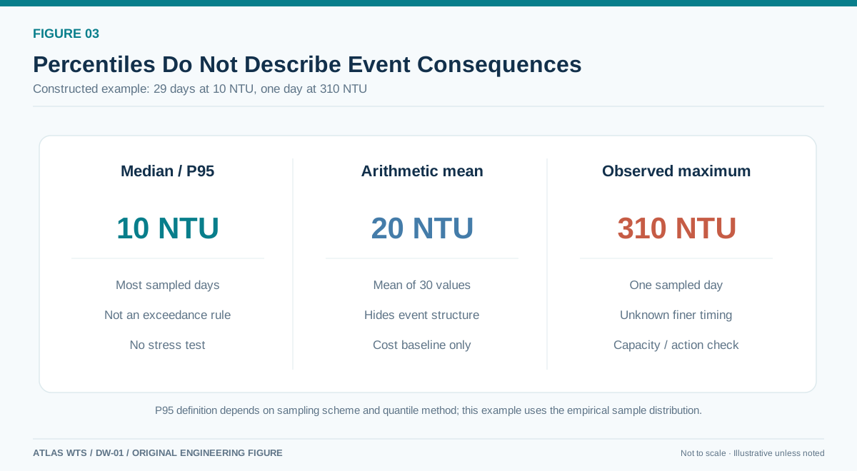
Figure 3 | P95 can remain low even when a rare high-magnitude event controls treatment capability.
Duration may matter more than a peak
Suppose a plant can temporarily increase coagulant dose, but its chemical inventory supports that high-dose operation for only 24 hours. Even if peak-hour treatment works, a 72-hour event may create a supply and operating failure.
Likewise, a filter may tolerate a brief increase in solids load but lose required backwash and standby capacity under several days of sustained loading.
A more informative event description is:
Event = peak + duration + rise rate + recovery time + concurrent conditions
A single maximum cannot express this.
05 | Why Not Combine All Individual Parameter Maxima?
One common “conservative” approach selects maximum turbidity, maximum DOC, minimum temperature, minimum alkalinity, maximum ammonia and maximum design flow from historical records and puts them together as one “worst case.”
That can cause both overdesign and overlooked risk.
First, these extrema may come from different seasons and hydrological regimes and may not be physically capable of occurring together. A combination without a plausible mechanism produces a fictitious super-event.
Second, a truly limiting combination may contain no individual maximum. Moderate turbidity with a high algal cell load may be harder for certain processes than very high mineral turbidity; cold water coincident with increased disinfectant demand may govern contact-time requirements.
Engineers should examine joint distributions and conditional relationships, not simply stack univariate extremes.
A sensible sequence is to align samples by location and time; investigate lag relationships; classify seasons and events; examine scatterplots, dependence, conditional quantiles and unusual combinations; define representative physically meaningful conditions; and stress-test rare but potentially severe combinations separately.
Statistical correlation does not prove causation. Nor does the absence of coincident historical maxima prove that such a combination can never occur.
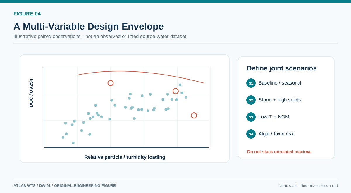
Figure 4 | Build a design envelope around evidence-supported joint conditions rather than a fictional combination of unrelated single-parameter extrema.
With long, high-frequency records, clustering, joint probability and conditional quantiles can help identify regimes. With limited records, hydrology, catchment knowledge and operating experience become even more important. Statistics organize evidence; they do not replace engineering interpretation.
06 | How To Build A Defensible Design Raw-Water Quality Envelope
This is the article’s central engineering procedure.
The envelope is not a min/mean/max table, but a design basis linking source-water risk, demonstrated treatment capacity and operating decisions.
The live ATLAS Municipal Drinking Water Purification Workflow places Source Water Characterization at the start of the train. Flow, chemistry and source-water quality boundaries must be established before downstream barriers are selected. The order matters: process selection should follow, not precede, the design basis.
Work backward from finished-water objectives
Before interpreting raw water, identify applicable regulations, permits and local requirements; pathogens, chemical pollutants and aesthetic objectives; proposed barriers and validation needs; supply rates, redundancy and acceptable interruptions; and principles for responding to intake excursions, equipment failure or loss of source supply.
A contaminant with a low long-term mean can still merit a dedicated scenario if it creates a critical finished-water hazard.
Build a traceable data foundation
Combine historical water quality, online instruments, laboratory results, actual intake flow, meteorological and hydrological events, plant logs and known upstream hazards.
Preserve time, location, analytical method, unit, detection limit, quality status and source version for each observation.
For parameters controlling design, check coverage of all important seasons, known high-risk events, relevant intake depths and alternative intakes, flow conditions associated with design, and enough consecutive observations to establish duration.
Document missing information in a design risk register and plan additional monitoring, jar tests, pilot studies or other verification. Do not silently replace gaps with a single empirical number.
Identify the mechanisms that actually govern capacity
Link each monitored indicator to treatment failure modes. Particle loading may govern sludge withdrawal and filter cycles. Organic character may control coagulation, adsorption competition and DBP risk. Cold water may limit flocculation or disinfection CT. Intracellular versus dissolved cyanotoxin fractions may change the chosen treatment sequence. Ammonia and reducing species may increase oxidant demand. Certain micropollutants may require dedicated removal barriers.
Not every parameter merits a separate scenario. Prioritize variables that change equipment size, process choice, operating range or emergency decisions.
Define a representative scenario matrix
This is an illustrative organizing framework, not measured data from one source and not a mandatory list for every plant.
| Scenario | Main characteristic | Potential limiting processes | Response to validate |
|---|---|---|---|
| S0 Normal | Typical seasonal quality | Routine chemical/energy use, stability | Normal operating window |
| S1 Storm shock | Higher turbidity and solids | Coagulation, clarification, filtration, sludge | Peak and sustained loading |
| S2 Algal bloom | Cells, taste/odor or toxin risk | Intake, cell removal, adsorption, oxidation | Toxin fraction and effective barriers |
| S3 Cold water | Altered reaction kinetics | Flocculation, filtration, disinfection | Low-temperature performance and CT |
| S4 Drought/concentration | Higher dissolved constituents | Specialized removal, blending, corrosion/scaling | Treatment limits and backup supply |
| S5 Abnormal contamination | Unusual pollutant or spill | Monitoring, isolation, intake shutdown | Recognition, warning, emergency action |
For every scenario, specify joint input conditions, duration, data confidence, treatment capability, operating strategy and exit criteria.
Split the envelope into three levels
Normal Operating Envelope: conditions under which the plant is expected to run sustainably within routine SOPs. Use this range to optimize chemicals, energy, utilization and maintenance.
Validated Upset Envelope: conditions supported by tests, operational records or comparably strong evidence for which adjusted chemical feed, flow, number of trains, backwash frequency or other controls maintain finished-water objectives.
Beyond-Validated Envelope: raw-water conditions beyond demonstrated treatment capability. Do not assume finished water remains safe by “adding more chemical” or “loading equipment harder.” Instead follow pre-defined flow reduction, intake shutdown, alternative supply, balancing, additional sampling or public-health contingency procedures.
These levels are more operationally useful than a single “maximum design value.”
Transfer each scenario into every downstream unit
Each unit should receive at least four items: design input, acceptable output, validation basis and exceedance action.
A clarifier or filter cannot work from “design turbidity: 100 NTU” alone. It needs particle properties, flow, duration, acceptable outlet turbidity, sludge withdrawal conditions and filter redundancy strategy.
A carbon adsorption unit likewise needs competing organic loading, breakthrough criteria, demonstrated capacity and media-replacement strategy—not only the contaminant peak.
Close uncertainty through testing and operating evidence
The envelope must be verifiable. Coagulation needs jar or appropriate pilot testing; membrane filtration needs sustainable flux, fouling, backwash and recovery tests; adsorption needs capacity and breakthrough data under relevant water quality; and disinfection needs effective contact-time assessment under applicable regulatory and hydraulic conditions.
Sizing tools help build preliminary material balances and equipment estimates, but are not substitutes for this verification.
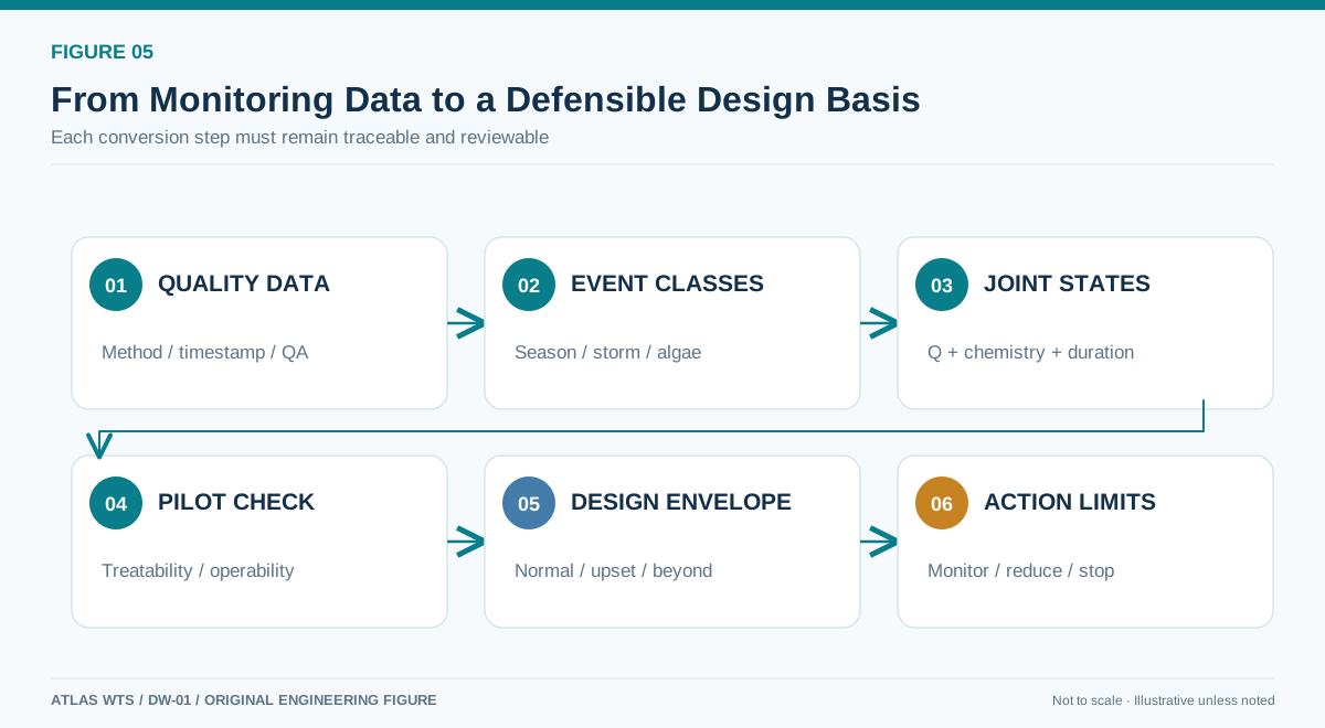
Figure 5 | A traceable loop from monitoring data to representative scenarios, equipment constraints, operating windows and exceedance actions.
07 | How The Source-Water Envelope Changes The Entire Treatment Train
An envelope is useful when it converts uncertain source variation into process constraints that can be evaluated, calculated and tested.
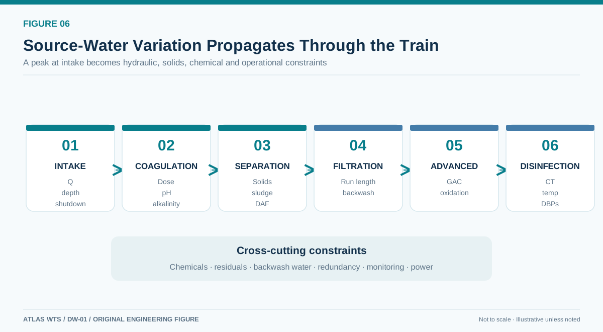
Figure 6 | Source-water scenarios do not remain in a water-quality report. They propagate through coagulation, separation, advanced treatment, disinfection and supporting systems.
Coagulation and conditioning: control the reaction window
Coagulant demand depends not only on turbidity but on particle surface properties, DOC, pH, alkalinity, temperature and removal objectives. A threefold turbidity increase does not automatically imply a threefold dose increase; dose response requires jar tests, piloting or reliable operational evidence.
Once candidate doses have been established for defined scenarios, chemical supply can be quantified.
ATLAS constructed example: plant flow = 50,000 m³/d; effective chemical constituent dose = 15 mg/L at normal operation and 45 mg/L during a validated upset.
M [kg/d] = Q [m³/d] × D [mg/L] / 1,000

Normal: 50,000 × 15 / 1,000 = 750 kg/d
Upset:  50,000 × 45 / 1,000 = 2,250 kg/d
If the commercial product contains 40% active constituent by mass and its density is 1.35 kg/L:
V_product [L/d] = M_active / (mass fraction × density)

Normal: 750 / (0.40 × 1.35) = 1,389 L/d
Upset: 2,250 / (0.40 × 1.35) = 4,167 L/d
Switching from normal to upset dosing therefore increases commercial-product consumption by approximately 2.78 m³/d.
These are calculation examples, not dose recommendations for an operating plant. A project must align active-content definitions, product strength, density and metering basis, then check storage tanks, pumps, piping, unloading and replenishment cycles.
ATLAS’s Chemical Dosing Basis Calculator can organize preliminary relationships between flow, dose and commercial product strength, but doses must still come from project-specific tests or experience.
Clarification and filtration: recovery as well as instantaneous capacity
Storms may rapidly increase solids loading.
With a measured TSS concentration, a preliminary incoming solids mass can be calculated:
Solids load [kg/d] = Q [m³/d] × TSS [mg/L] / 1,000
This is incoming suspended solids, not final sludge dry solids. Coagulant precipitates, actual removal fractions and other sources change the residuals balance.
For clarifiers, examine overflow rate, solids flux, withdrawal capacity and short-circuiting risk. For filters, evaluate run length, terminal head loss, backwash demand and recovery after washing.
For UF/MF, assess fouling rate, sustainable flux, backwash water use, chemically enhanced backwash and available trains.
A simplified membrane-flux sensitivity example illustrates the importance. For instantaneous treatment flow of 2,083 m³/h, neglecting backwash downtime, recovery losses and spare capacity:
A [m²] = Q [L/h] / J [L/(m²·h)]

J = 65 LMH → A ≈ 2,083,000 / 65 = 32,046 m²
J = 45 LMH → A ≈ 2,083,000 / 45 = 46,289 m²
The latter area is approximately 44% larger.
This is not a final membrane design: net yield, backwash, CEB, spare trains, recovery and fouling allowances have not been included. The point is that sizing membrane area from average water quality alone may be materially wrong if sustainable flux under adverse raw-water conditions is unknown.
ATLAS UF/MF System Designer can support preliminary membrane area, train, backwash and recovery estimates.
Adsorption and oxidation: contaminant form governs barrier effectiveness
Organics, cyanotoxins, taste/odor compounds and specific micropollutants may require adsorption or oxidation, but these technologies are not interchangeable universal remedies.
PAC and GAC have different design questions. PAC requires feed location, mixing, contact time, downstream solids separation and sludge loading. GAC requires EBCT, competitive adsorption, breakthrough curves, bed hydraulics and media replacement.
The ATLAS Activated Carbon Sizing tool supports preliminary fixed-bed calculations; it should not be used to infer optimal PAC field dose.
Oxidation also requires a clear target. For algae-bearing water, removing intact cells, avoiding cell rupture and managing dissolved toxins are distinct objectives. Some preoxidation conditions can alter cell integrity and contaminant speciation. Verify process sequencing under representative conditions.
For ozone, consider actual oxidant demand, mass transfer, residual, effective contact time and byproduct risks such as bromate where relevant, not just the applied dose. ATLAS Ozone Dosing & CT Screening provides preliminary screening, not a substitute for regulator-accepted contact-time validation.
Disinfection: raw-water variability influences microbial barriers
Disinfection cannot be based on a single theoretical contact time at room temperature.
Where CT assessment is applicable, residual disinfectant, effective contact time, temperature, pH, target microorganisms and reactor hydraulics determine performance. Applicable local rules govern calculation and validation.
For example, US surface-water rules include combined filter effluent treatment-technique turbidity limits for covered conventional and direct filtration systems: at least 95% of relevant measurements per month must be at or below 0.3 NTU, and no such measurement may exceed 1 NTU. Coverage depends on system category and legal requirements; these are not universal global limits. US EPA Surface Water Treatment Rules
An envelope is meant to maintain finished-water and public-health objectives across the whole train, not simply show that one unit can handle high turbidity.
Plant-wide systems: chemicals, residuals, hydraulics and redundancy
The same scenario matrix should inform chemical storage and metering; sludge thickening, dewatering and disposal; backwash water and drains; flow balancing and clearwells; minimum supply with one train offline; automation, alarm and event logging; and the ability to restrict or suspend intake.
Some limiting failures occur not in the main process units but in supporting equipment not designed for the same upset scenario.
A complete ATLAS hypothetical scenario calculation
Extend Source A’s storm day into a clearly identified instructional example, not data from a real facility.
| Parameter | Normal condition | Storm upset | Design implication |
|---|---|---|---|
| Flow | 50,000 m³/d | 50,000 m³/d | No flow reduction assumed |
| Turbidity | 10 NTU | 310 NTU | Optical particle indicator only |
| TSS | 12 mg/L | 220 mg/L | Separate assumption; not derived from NTU |
| Effective-constituent chemical dose | 15 mg/L | 45 mg/L | Assumed validated by testing |
| Event duration | Normal | 24 h | Chemical stocks and residuals capacity |
Incoming suspended-solids loading:
Normal: 50,000 × 12 / 1,000 = 600 kg/d
Storm:  50,000 × 220 / 1,000 = 11,000 kg/d
Thus incoming TSS mass increases from 0.6 to 11 t/d—approximately 18 times the normal load. Effective chemical demand concurrently rises from 0.75 to 2.25 t/d.
Neither change is conveyed by an average turbidity of 20 NTU. Even with unchanged instantaneous clarifier hydraulic loading, sludge withdrawal, storage, dewatering, chemical deliveries and filter backwash may increase considerably.
If storms could persist for 72 hours, the team must also check:
Active constituent for 72 h upset = 2.25 t/d × 3 d = 6.75 t
Incoming TSS over 72 h         = 11 t/d × 3 d = 33 t
The 33 t is incoming TSS, not dewatered sludge mass. Actual residuals include coagulant precipitates, removal rates, solids concentration and other sources.
The envelope converts a water-quality event into the mass and time demands that equipment and operations must actually carry.
08 | Real Case: What Does The 2014 Toledo Cyanotoxin Incident Teach Us?
Location: Toledo, Ohio, United States
Source: Lake Erie
Primary issue: bloom-related microcystins rapidly changed treatment and public-health decision conditions.
Only public event facts and values from the US EPA report are cited here. The engineering interpretation is ATLAS’s own and is not an EPA recommendation for that facility’s future design conditions.
What happened in raw and finished water?
According to the EPA cyanotoxin management recommendations, microcystin at Toledo’s Lake Erie intake rose rapidly to 14 μg/L in early August 2014.
The EPA reports 2.5 μg/L in finished water, confirmed by repeat sample analysis by two different analysts. Ohio EPA then recommended a “Do Not Drink” advisory. Approximately 500,000 people were affected, and the advisory lasted 55 hours.
The data reveal two important points.
First, cyanotoxins are a separate control target; routine turbidity cannot reliably characterize their drinking-water risk.
Second, a critical contaminant may change rapidly. A low long-term average does not establish that the current operating condition can handle a sudden high-risk event.
What did the plant change?
The EPA reports treatment optimization after microcystin was detected in finished water, including raising powdered activated carbon dosing from 6.3 to 15 mg/L and increasing alum and chlorine doses.
Finished-water microcystin subsequently fell close to the detection limit, and the advisory was lifted.
6.3 → 15 mg/L must not be copied as a general PAC recipe: NOM, cell integrity, dissolved toxin fraction, contact time, carbon type and downstream separation vary by plant.
The design lesson is that operators need to know which controls are adjustable, the proven adjustment range, and how to verify finished-water performance after an intervention.
A higher raw-water concentration occurred afterward
The EPA reports that 11 days after the advisory ended, intake microcystin rose again to >50 μg/L, the highest in the preceding five years of monitoring.
The plant was already running enhanced microcystin treatment. Finished-water microcystin was again detected, but did not exceed the report’s then-cited 1.0 μg/L threshold.
Two distinctions are essential:
- “>50 μg/L” is a lower-bound statement, not an exact 50 μg/L measurement;
- “did not exceed 1.0 μg/L” is a threshold comparison, not a specific finished-water sample value.
It is invalid to divide 50 by 1.0 and claim an exact removal percentage, or fit a complete dose–removal model from these sparse public event facts.
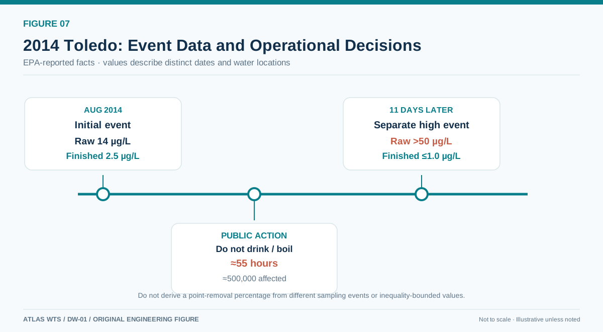
Figure 7 | Key event points reported by EPA and redrawn by ATLAS. Separate observations are not joined into a fictitious continuous time series.
From emergency response to longer-term capacity
The EPA describes later upgrades, including raising PAC system dosing capability to 40 mg/L, adding PAC feed locations and developing broader long-term process improvements. The report estimated an initial upgrade cost of about USD 4.4 million.
The 40 mg/L figure refers to planned future dosing capacity, not a dose documented during the event, nor a recommended dose for other plants.
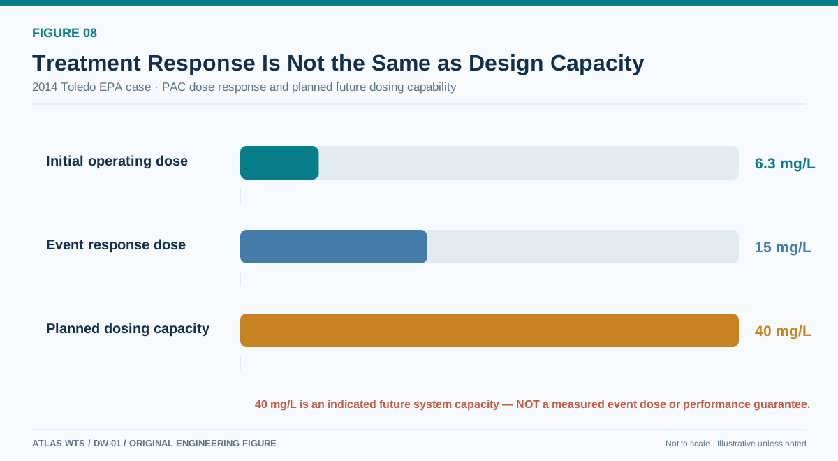
Figure 8 | EPA PAC values distinguish the reported pre-event dose, emergency response dose and later increased capacity. These represent different engineering quantities.
ATLAS interpretation: translating the event into a design basis
Toledo does not imply that every plant must design for >50 μg/L microcystin, nor do the published facts reconstruct the full hourly intake distribution.
The case nonetheless identifies five indispensable elements:
Contaminant identification. Turbidity, pH and generic organic measures may miss a source-specific cyanotoxin hazard.
Continued monitoring during abnormal conditions. The end of the first advisory did not mark permanent source-water recovery. A second, higher intake concentration argues for monitoring after apparent recovery and through repeated shocks.
Actually adjustable treatment capacity. PAC feed, contact, separation and other chemical processes require validated operating ranges—not merely normal doses.
Finished-water verification. Higher intake concentrations do not always translate into finished-water exceedances; lower intake concentrations likewise do not guarantee safety. Decisions require appropriate effluent testing and verification of barriers.
Exceedance decision-making. When raw water enters an unvalidated risk region, preplanned criteria must govern enhanced treatment, additional sampling, restricted supply and public-health action.
The design basis must encode more than a “maximum cyanotoxin concentration”:
Monitor → assess → treat → verify → recover / activate emergency response
The public Toledo values are discrete event records, not a complete hourly dataset. Therefore no Toledo P95, P99, annual average, continuous concentration curve or precise removal efficiency is fabricated here.
09 | Monitoring And Data Quality That Can Support Engineering Design
Even hundreds of thousands of records cannot guarantee a reliable design basis unless they cover the right questions.
Online instruments and laboratories perform different roles
Online instruments can capture fast changes, establish event triggers and reveal temporal patterns—turbidity, pH, temperature, conductivity and selected optical indices.
Laboratories confirm target contaminants, toxins, metal speciation, organic characteristics and regulatory analytes.
Surrogates can inform intensified sampling, but cannot replace verified laboratory measurement of a target contaminant. For example, chlorophyll-a can indicate algal activity, not directly quantify microcystin.
Routine sampling cannot substitute for event sampling
A 36-hour event can fall entirely between monthly sample dates.
Monitoring therefore needs distinct modes:
Routine monitoring: seasonal baselines and stable conditions.
Event-triggered monitoring: additional samples after storms, blooms, spills or online anomalies.
Verification monitoring: confirmation of treatment adjustments, tests and finished-water quality.
Recovery monitoring: evidence that the source and process have returned to the validated normal envelope.
Trigger criteria should be source- and risk-specific, not one global numeric threshold.
Missing data and detection limits must enter statistical analysis
Missingness in continuous monitoring may be nonrandom: outages, storms, fouling or overrange instruments can coincide with the most important periods.
Dropping those intervals before calculating means or percentiles can systematically understate risk.
Similarly, below-detection results cannot automatically be replaced with zero. Retain reporting limits and censoring flags, and select a treatment appropriate to the statistic.
Preserve original extreme records, QC outcomes and amendment histories. Do not delete a genuine peak merely to smooth a curve, nor incorporate an obvious instrument fault without review.
Data resolution must match response time
If an intake shock forms within 30 minutes, daily means cannot show whether chemical dosing control reacts fast enough.
Conversely, evaluating seasonal organic loads and adsorbent life may require distributions and cumulative mass more than minute-by-minute variation.
Choose sampling frequency by contaminant dynamics, equipment response and consequence. Resolution should support the decisions operators actually need to make.
Modern plants must also engineer data integrity: synchronized timestamps, sensor calibration, event tags, laboratory method versions, anomaly review, missing-data causes and operating logs.
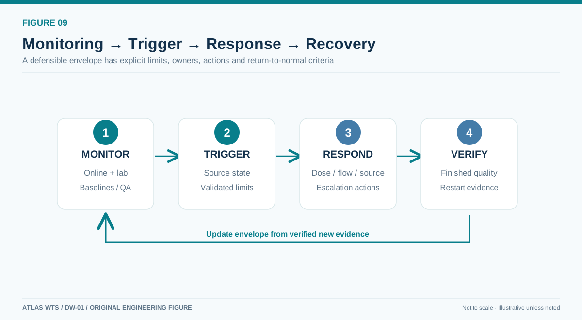
Figure 9 | The source-water envelope is not static. Monitoring, triggers, field verification, process or intake response and recovery checks form a closed decision loop. Original ATLAS methodology.
10 | Frequent Design Errors And Project Audit Checklist
Selecting equipment from annual average quality alone
Annual averages describe overall levels, not event scenarios, extreme loads or recovery capability.
Treating the historic maximum as the only design point
A maximum does not describe duration or automatically predict future extremes. Examine QC, physical mechanism and assigned engineering response.
Mechanically stacking parameter maxima
This can create unsupported combinations while hiding the conditions that truly govern process capacity.
Treating online surrogate indicators as target contaminant measurements
Turbidity, UV254 and chlorophyll-a are useful, but cannot replace unvalidated tests of cyanotoxins, pathogens or specific chemicals.
Checking primary treatment units but not supporting systems
Chemical inventory, dosing pumps, sludge withdrawal, backwash water, backup power and controls may be the limiting equipment under upset conditions.
Treating calculator outputs as guaranteed performance
Preliminary computations expose sizing and balance questions, not a substitute for testing, vendor verification, regulatory review or accountable design judgment.
Failing to define action outside the design envelope
A particularly hazardous design document claims it can handle “all abnormal raw water” but defines neither a validated limit nor an exceedance response.
Project audit checklist
| Audit item | Minimum supporting evidence | Status |
|---|---|---|
| Finished-water goals and key contaminants defined | Regulations/permits and project targets | ☐ |
| Source records cover key seasons | Seasonal statistics, sampling calendar | ☐ |
| Known high-risk events represented | Storms, blooms, incidents | ☐ |
| Units and analytical methods traceable | Methods, instruments, units, detection limits | ☐ |
| Distinct mean and quantile definitions | Time-/flow-weighting, P50/P95/P99 | ☐ |
| Event duration analyzed | Peaks, duration, rise and recovery | ☐ |
| Joint parameter variation reviewed | Aligned records, conditional plots, rationale | ☐ |
| Three operating envelope levels established | Normal / Validated Upset / Beyond-Validated | ☐ |
| Scenarios propagated through all units | Unit design inputs and exceedance-action matrix | ☐ |
| Supporting systems checked under same scenarios | Chemicals, sludge, backwash, redundancy, power, controls | ☐ |
| Critical capacity backed by evidence | Jar tests, pilot data, operating evidence | ☐ |
| Event triggers and recovery defined | Alarms, sampling, switching, flow restriction, recovery criteria | ☐ |
| Unverified assumptions tracked | Data gaps, extra monitoring, test plan | ☐ |
The goal is not to tick every box formally, but to make every judgment traceable to evidence. The envelope is an auditable engineering decision chain.
11 | Conclusion: A Design Basis Should Be An Executable Decision System
Average raw-water quality has legitimate uses: characterizing long-term conditions, comparing sources, estimating some mean loads and describing normal operations.
The problem starts when an average is treated as the complete design basis. Important source behavior—variability, event duration, parameter dependence, treatment response and recovery—is then lost.
A stronger approach establishes a multidimensional, validated scenario system that can be passed through every treatment process.
It must answer how the source changes in normal periods; which upset events govern treatment; which variables must be considered jointly; under which conditions each barrier can meet its targets; what validated adjustments operators can make; whether chemicals, residuals, backwash, backup electricity and automation support those adjustments; and how supply is protected beyond demonstrated capacity.
Toledo 2014 shows that reliability does not depend on picking a sufficiently large “maximum contaminant concentration” alone. It depends on recognizing hazards in time, adjusting treatment, verifying outcomes and, if necessary, implementing clear public-health and supply actions.
A good raw-water design basis is not a static water-quality table. It is an engineering system connecting monitoring evidence, treatment capacity and operational decisions.
The key starting question for any drinking-water project entering process selection, equipment sizing or detailed design is not:
“What is the average raw-water quality?”
It is:
“Under which reasonably foreseeable future source-water conditions can we demonstrate, with evidence, that this plant will remain reliable?”