The Water Treatment Challenge Behind the AI Data Center Boom: How Cooling Architecture, Reclaimed Water, Cycles of Concentration and Brine Management Define Hyperscale Water Use

The AI water question is usually framed too narrowly

The question “how much water does an AI data center use?” sounds simple, but it is usually the wrong engineering question. Water demand is not a fixed attribute of compute. It emerges from a chain of decisions: rack density and chip temperature, direct-to-chip versus air cooling, the final heat-rejection architecture, local dry-bulb and wet-bulb conditions, the quality of the available makeup water, the number of times that water can be concentrated safely, the treatment required to make that concentration possible, and the fate of the blowdown or membrane concentrate left behind.

That systems view is becoming increasingly important. The U.S. Environmental Protection Agency’s Water Reuse Action Plan 2.0, released in April 2026, explicitly includes an action to help states expand recycled-water use for industrial and data-center cooling. The Water Research Foundation is separately studying both fit-for-purpose industrial reuse and non-evaporative cooling. Water is no longer just an ESG line item for data-center operators; it is now a siting, utility-planning, permitting and thermal-design constraint.

At the same time, the scale of the electricity system behind AI is moving quickly. Berkeley Lab’s 2025 update to U.S. data-center energy use estimates that data centers could account for about 11.8% of U.S. electricity consumption by 2030, with a scenario range of 9.5%–15.3%. A separate Berkeley Lab review of water use at the workload level found variation exceeding 10,000-fold, driven by server efficiency, grid water intensity, utilization, cooling technology, facility efficiency, climate and other variables. There is therefore no defensible universal number for “liters of water per AI workload” that can be separated from location and architecture.

This article develops a common engineering model around a 300 MW continuous IT load and uses three representative U.S. locations—Northern Virginia/Loudoun, Dallas–Fort Worth and Phoenix—to expose the mechanisms. The model is intentionally transparent about what is measured and what is assumed. The wet-heat-rejection shares, illustrative makeup-water chemistry and several membrane-recovery values are engineering scenarios, not disclosed operating data from real hyperscale campuses. Their purpose is to compare mechanisms and orders of magnitude, not to replace twelve months of source-water analysis, hourly weather files, vendor membrane projections or permit review.

The central conclusion is simple:

The best water-treatment strategy for a new AI campus is usually not to find more water first. It is to minimize the amount of heat that must be rejected through evaporation, then design fit-for-purpose water treatment for the wet-cooling load that remains.

That is also the logic behind the site’s broader Data Center Cooling & Water Strategy: thermal architecture belongs upstream of the water plant.

A 300 MW reference model: where the water demand begins

The model assumes a continuous 300 MW IT load for 8,760 hours per year:

$$E_{IT}=300\ MW\times 8{,}760\ h=2.628\ TWh/y$$

For the wet-cooling comparison, the average heat-rejection duty is set at 330 MW, or IT load multiplied by 1.10. Using a water-vapor latent heat of approximately 2.43 MJ/kg, equivalent to about 0.675 kWh/kg, the annual evaporation if 100% of that heat were rejected evaporatively is:

$$E_{100\%} = \frac{330{,}000\ kW\times8{,}760\ h} {0.675\ kWh/kg} \approx4.283\times10^9\ L/y = 4.283\ GL/y$$

The comparison then assigns annual wet-heat shares of 60% in Northern Virginia, 75% in Dallas–Fort Worth and 90% in Phoenix:

$$E_{site}=4.283\times f_{wet}$$

Site	Assumed annual wet-heat share	Annual evaporation	Evaporation-only WUE
Northern Virginia	60%	2.57 GL/y	0.98 L/kWh-IT
Dallas–Fort Worth	75%	3.21 GL/y	1.22 L/kWh-IT
Phoenix	90%	3.85 GL/y	1.47 L/kWh-IT

These are not actual WUE values for operating facilities in those locations. They are a wet-cooling exposure baseline. Real hyperscalers have already demonstrated far lower fleet-level WUE through different architectures. Microsoft reported that its average WUE fell from 2.3 L/kWh in early generations to 0.27 L/kWh in 2025, while AWS reports a global data-center WUE of about 0.12 L/kWh. Microsoft also describes closed-loop, direct-to-chip designs that use zero water evaporation for cooling. ASHRAE’s 2026 AI Data Center Framework states that direct-to-chip liquid cooling has become an industry standard for AI/HPC and that warm-water, chiller-less designs can enable near-zero cooling-water use in many climates.

Those public benchmarks do not invalidate the tower model. They clarify what the model is for: it is a traditional wet-rejection comparison baseline, useful for understanding what happens when a large fraction of the campus heat still enters an evaporative system.

Why public WUE is a benchmark, not a 300 MW design input

Fleet WUE is valuable as a reality check, but it is not a substitute for the water balance of a specific site. A reported corporate WUE normally reflects a defined reporting boundary across many facilities, climates and cooling configurations. It can include sites that use water only during extreme weather, sites that operate mostly dry, leased capacity, and equipment generations with very different cooling strategies. A project-level process model needs to know something more specific: how many megawatts of heat enter an evaporative device during each hour of the year, and what water stream supports that device.

This distinction matters because two facilities with the same annual WUE can have very different infrastructure needs. One may use a small amount of water continuously; another may use almost none for nine months and then require a large peak flow during the hottest weeks. The annual liters-per-kWh number can be identical while the required water-main capacity, storage volume, cooling-tower cells, blowdown permit and treatment peak are completely different.

A useful design therefore separates at least four quantities:

$$\text{annual water consumption}$$ $$\text{peak makeup flow}$$ $$\text{peak blowdown / concentrate flow}$$ $$\text{seasonal chemistry at the peak-flow condition}$$

The last item is often the one that gets missed. The most water-intensive hour may also be the hour with the warmest circulating water, the highest biological activity, the highest approach temperature and the most aggressive corrosion environment. If a reclaimed-water source also experiences seasonal chloride, ammonia or TOC excursions, the worst hydraulic condition and worst chemistry condition can coincide.

The same caution applies to water replenishment metrics. Replenishment is important watershed stewardship, but it does not replace the process engineering question. A project can replenish water elsewhere and still need a reliable local water source, a pipe sized for the summer peak and a legal outlet for concentrated blowdown. Watershed accounting and cooling-water design answer different questions.

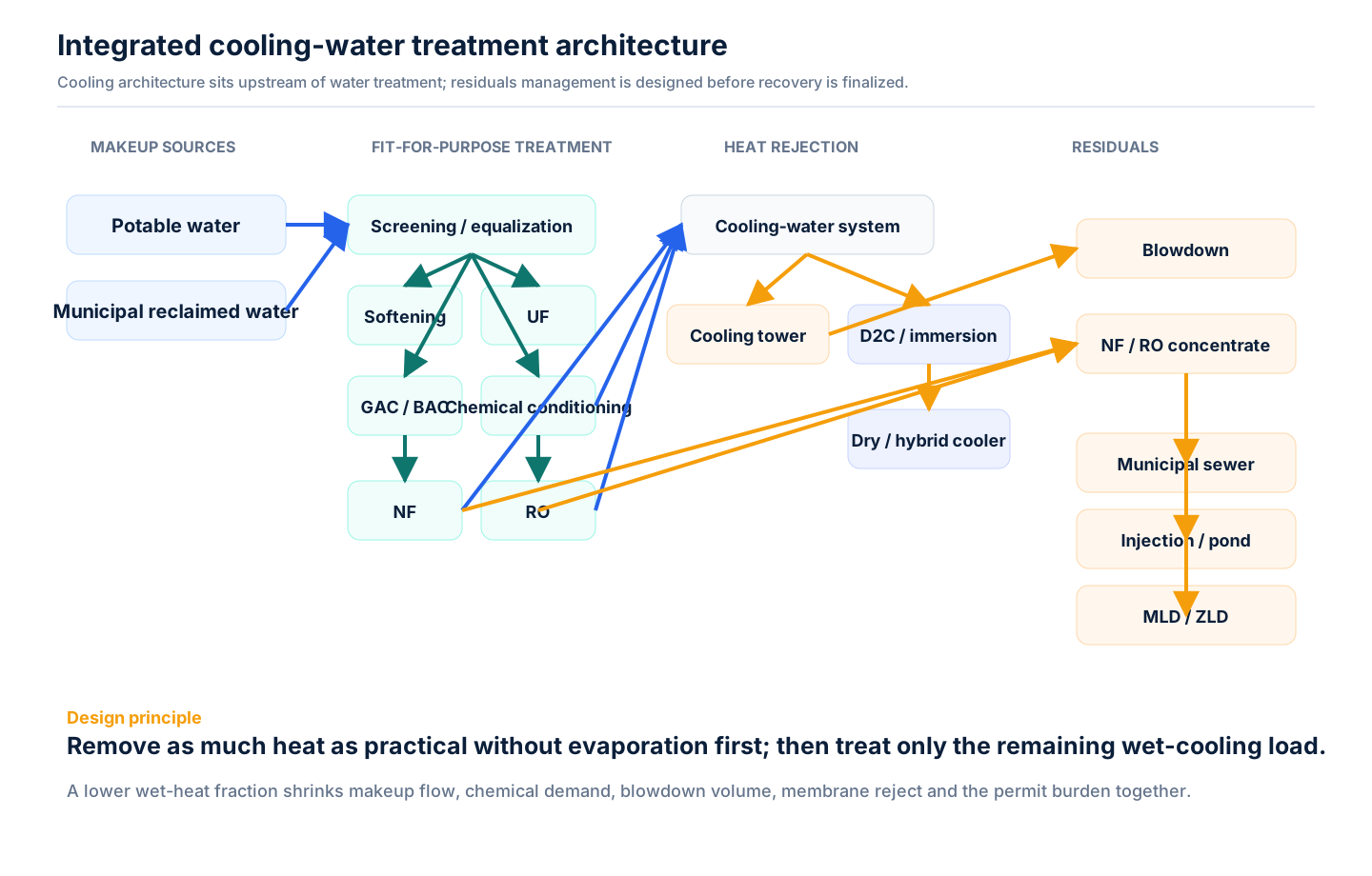
Integrated process model. The critical design decision appears before the water-treatment train: how much heat should enter an evaporative loop at all?

Three boundaries are needed: site water, source water and discharge

A meaningful water analysis needs at least three boundaries.

Boundary A — site water

The familiar facility boundary is:

$$W_{site} = W_{cooling} + W_{humidification} + W_{domestic} + W_{treatment\,loss}$$

For large AI facilities, cooling and treatment losses dominate the engineering discussion, but the definition matters because a treatment train can increase withdrawals even while improving the chemistry of the water that reaches the tower.

Boundary B — source water

The wider boundary adds water consumed upstream in power generation:

$$W_{source} = W_{site} + E_{facility}\times I_{grid,water}$$

where $I_{grid,water}$ is the water-consumption intensity of the electrical supply. Berkeley Lab’s workload analysis is important because grid water consumption is one of the highest-ranked determinants of workload water use. A facility can drive onsite evaporation toward zero and still carry a non-zero upstream water footprint through electricity. Conversely, the extra source-water burden of dry/mechanical cooling can still be much smaller than several gigaliters per year of direct evaporation. It must be calculated, not assumed.

Boundary C — watershed and discharge

The third boundary is what leaves the water system other than vapor:

$$W_{residuals} = W_{blowdown} + W_{RO/NF\,reject} + W_{regeneration\,waste} + W_{chemical\,residuals}$$

This is the boundary that separates genuine water avoidance from problem-shifting. A design may reduce freshwater withdrawal while creating a chloride-rich blowdown, or it may stabilize cooling chemistry with RO while creating a separate membrane concentrate that needs sewer capacity, injection, evaporation, MLD or ZLD.

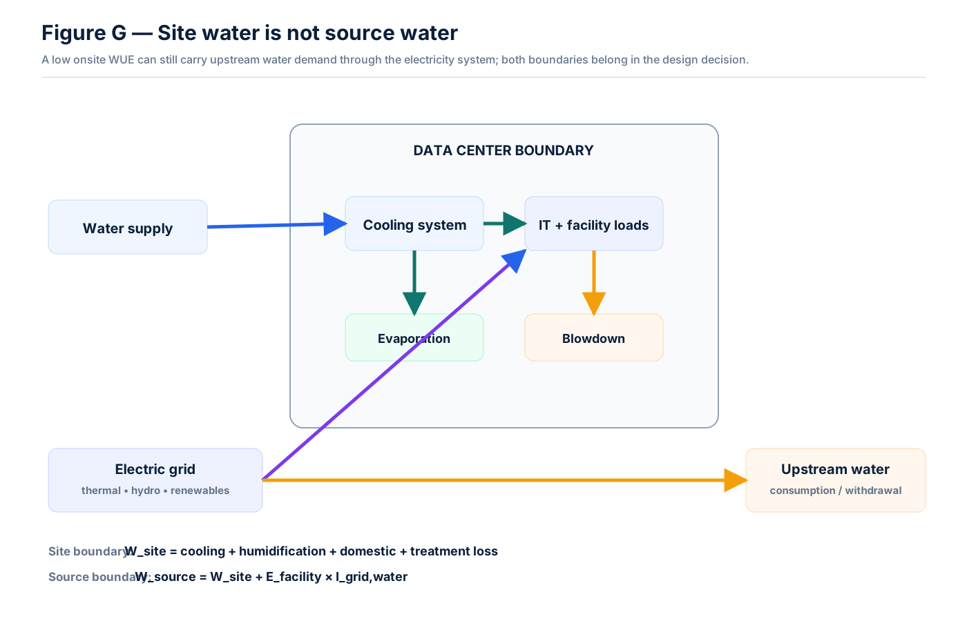
Figure G — Site water is not source water. WUE at the property line is necessary, but it is not a complete lifecycle water metric.

Why AI changes the cooling decision before it changes the water plant

High-density AI racks are pushing thermal design away from the assumption that room air is the primary heat-transport medium. Four broad architectures matter for this discussion.

Cooling architecture	Site water use	Cooling energy	Climate sensitivity	AI heat-density capability	Water-treatment implication
Air cooling + chiller/dry rejection	Low	Medium–high	High in hot weather	Limited at extreme rack density	Relatively simple open-water chemistry; higher mechanical cooling burden
Evaporative cooling / cooling tower	High	Often low	Strongly wet-bulb dependent	Depends on secondary cooling architecture	Highest open-water burden: scale, corrosion, biofouling, blowdown
Direct-to-chip + CDU	Depends on final heat rejection; near-zero with dry rejection	Low	Warm-water design can reduce climate penalty	High	Closed-loop coolant chemistry plus any remaining open-tower chemistry
Immersion + dry rejection	Very low	Low	Relatively low	Very high	No open IT-side water path; dielectric-fluid and heat-exchanger compatibility become important

ASHRAE’s current framework treats power and cooling as one system and explicitly describes warm-water D2C as a route to chiller-less dry heat rejection. Microsoft’s experience shows the same tradeoff from an operator’s perspective: eliminating evaporation can increase mechanical-cooling energy, but higher coolant temperatures provide more economizer hours and reduce the penalty. The right conclusion is therefore neither “water cooling is always greener” nor “zero-water cooling is always greener.” The conclusion is that heat rejection must be optimized against both water and energy constraints at the site actually being designed.

Warm-water liquid cooling changes the problem; it does not make water chemistry disappear

Direct-to-chip cooling is sometimes described as if it removes “water treatment” from the data center. That is only true if the phrase is restricted to an open evaporative loop. D2C actually creates two different water-chemistry regimes that must not be confused.

On the IT side, the coolant is typically a closed recirculating fluid serving cold plates through a CDU. The chemistry is much more stable than a cooling tower because there is no intentional evaporation, but the consequences of poor chemistry can be severe: corrosion products, galvanic interactions, elastomer compatibility, oxygen ingress, particulate contamination and biological growth can all threaten narrow channels and high-value cold plates. The correct program is therefore not “tower chemistry with a lower dose.” It is a closed-loop materials and coolant-compatibility program with controlled water quality, inhibitor chemistry and cleanliness.

On the facility side, the heat still has to leave the building. If it leaves through a dry cooler, site evaporative water can approach zero. If the dry cooler uses adiabatic trim during extreme conditions, water becomes an intermittent peak utility rather than a continuous base utility. If the D2C loop ultimately rejects heat to an open cooling tower, the campus still has all of the scale, corrosion, microbiological and blowdown constraints discussed in this article—the liquid cooling simply moved heat more efficiently from the chip to the facility water system.

This separation is important for project scope. A “liquid-cooled data center” is not automatically a “waterless data center.” The final water demand is controlled by the last heat-rejection step, while the reliability of the IT liquid loop is controlled by a different chemistry envelope. Treating those as one generic water system creates poor specifications on both sides.

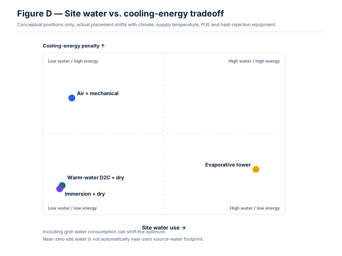
Figure D — Conceptual water–energy quadrant. Positions are directional, not industry-average measurements.

Cooling towers are water-chemistry reactors, not just heat exchangers

Once a design retains evaporative cooling, cycles of concentration (COC) becomes one of the most important control variables linking water quantity to chemistry.

Neglecting drift and leakage for a well-maintained system:

$$COC\approx\frac{M}{B}$$ $$B=\frac{E}{COC-1}$$ $$M=E+B=E\frac{COC}{COC-1}$$

where $M$ is makeup, $E$ is evaporation and $B$ is blowdown. The U.S. Department of Energy notes that many cooling systems operate around 2–4 COC, while 6 or higher can be possible with appropriate water treatment. Moving from COC 3 to 6 cuts makeup by about 20% and blowdown by about 50%.

The equations also show why chasing the highest possible COC is usually a poor optimization target. For a fixed evaporation load:

COC	Makeup / Evaporation	Blowdown / Evaporation
2	2.000	1.000
3	1.500	0.500
4	1.333	0.333
5	1.250	0.250
6	1.200	0.200
8	1.143	0.143
10	1.111	0.111

From COC 3 to 5, makeup falls by about 16.7% and blowdown falls by 50%. From COC 5 to 8, makeup falls only another 8.6%. Water savings flatten rapidly.

Chemistry does not flatten. For a conservative dissolved constituent with no precipitation, biodegradation, gas exchange or reaction:

$$C_{circulating}\approx C_{makeup}\times COC$$

Chloride and sodium often behave closest to this ideal. Calcium, bicarbonate and sulfate deviate once minerals begin to precipitate. Bicarbonate also responds to carbon-dioxide stripping and pH. Ammonia may nitrify or strip. TOC may biodegrade, oxidize or adsorb. Silica can polymerize or co-precipitate and interact with Mg/Al. The linear relation is therefore a screening upper bound, not a prediction of a real reacted cooling-water sample.

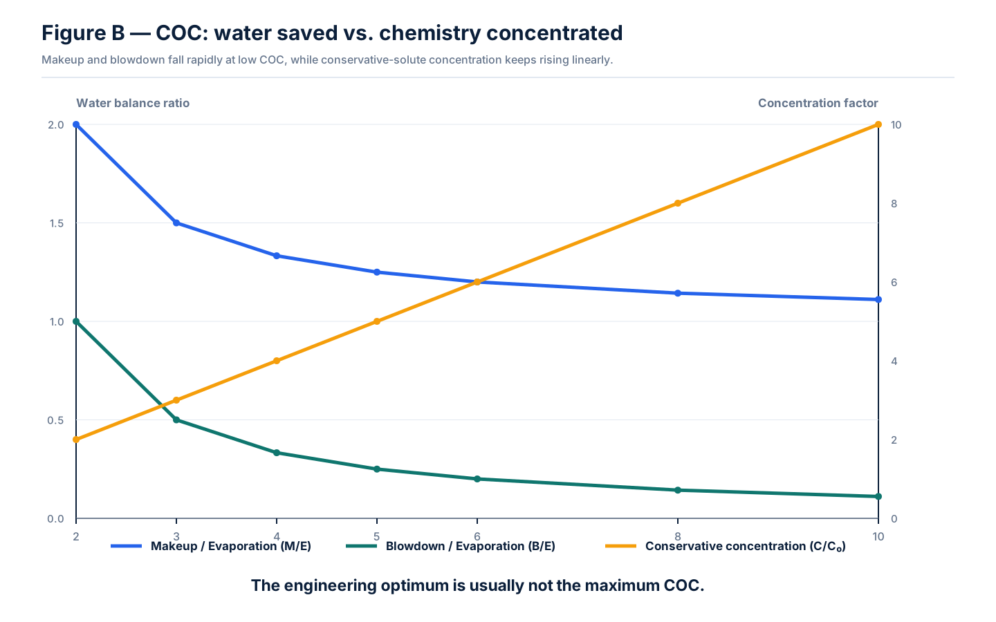
Figure B — The core tradeoff. Water savings flatten; chemical concentration does not.

This is also where the site’s Cooling Tower Water Balance & LSI Calculator becomes directly useful: the mass-balance side and the scaling/corrosion side must be evaluated together rather than as separate design tasks.

What actually happens to the major ions as concentration increases

The screening equation $C_{circulating}\approx C_{makeup}\times COC$ is deliberately conservative, but each major water-quality parameter eventually departs from it for a different reason.

Calcium and alkalinity are coupled through carbonate equilibrium. As water evaporates, calcium and bicarbonate concentrate, while air–water contact strips CO₂ and can shift pH upward. The carbonate saturation state may therefore increase faster than a simple TDS multiplier suggests. Once CaCO₃ begins to precipitate, dissolved calcium no longer follows the linear concentration line because part of the mass has moved to a solid surface. The practical question becomes not “what is the dissolved calcium?” but “where is the calcium going, at what rate, and on which heat-transfer surface?”

Sulfate can remain conservative at modest concentration, then become limited by gypsum or other sulfate scales depending on calcium, temperature and ionic strength. This is one reason selective softening ahead of a tower or membrane can have disproportionate value: removing a divalent cation can raise the allowable concentration of several anions downstream.

Silica is especially awkward because there is no single universal “silica limit.” Solubility and polymerization depend on pH, temperature, residence time and the presence of magnesium, aluminum and other surfaces. A number such as 100 mg/L can be useful as a screening warning in legacy design guidance, but it should never be treated as a material-independent pass/fail threshold. At high COC, silica is often the parameter that turns an apparently attractive water balance into a pilot-testing problem.

Chloride is different. It is usually close to conservative because it does not conveniently precipitate under normal cooling-water conditions. That makes it an excellent tracer for concentration, but also a corrosion concern. The safe chloride concentration depends strongly on metallurgy, temperature, oxidant residual, crevices, deposits and the selected corrosion inhibitor. A carbon-steel system, a 304 stainless exchanger and a high-alloy stainless system do not share one chloride ceiling.

TOC, ammonia and nutrients are not scale-forming salts, but at high concentration they can make the microbial program more difficult. Reclaimed water with very low TSS can still be biologically challenging if biodegradable organics or ammonia are present. Nitrification changes alkalinity and oxygen demand; biofilm changes local pH and ORP; oxidant demand changes the residual needed to control Legionella risk. This is why a reclaimed-water specification that lists only turbidity and TDS is incomplete for a cooling application.

The result is a practical rule: COC is not one number. It is the lowest allowable concentration factor imposed by all of the active chemistry and material constraints at the same time. One site may be chloride-limited; another silica-limited; another limited by calcium carbonate, biological control or the sewer’s TDS permit.

The chemical ceiling of COC should be calculated from simultaneous constraints

In practice, a project team often asks for “the maximum COC” too early. There is no useful answer until the controlling constraints are placed on the same sheet. A tower can be below a calcium-carbonate scaling threshold and still be unacceptable because chloride has crossed a metallurgy-specific limit. A membrane-softened makeup may solve hardness while making silica the next ceiling. A reclaimed-water source may look comfortable on inorganic chemistry but become limited by ammonia, TOC and disinfectant demand during the warmest months.

A better screening procedure is to calculate, for each potential makeup source and treatment train, the maximum concentration factor implied by each independent constraint:

$$COC_{allowable} = \min\left( COC_{CaCO_3}, COC_{CaSO_4}, COC_{silica}, COC_{chloride}, COC_{biology}, COC_{permit}, \ldots \right)$$

The expression is conceptual—several of those terms require equilibrium, kinetics or empirical control models rather than a simple concentration ratio—but it forces the right design behavior. The tower should operate below the first constraint it actually reaches, not below an arbitrary industry COC target.

It also makes source treatment easier to optimize. If chloride is the limiting term, sodium-cycle softening will not solve the problem. If hardness is the limiting term and chloride still has large margin, NF or chemical softening may be more rational than full desalination. If biological control is limiting, removing hardness does little; GAC/BAC, oxidation strategy, nutrient control, filtration and water-age management may matter more. This is the engineering value of a chemistry ceiling: it tells the project which unit operation buys additional COC and which one merely makes the water “cleaner” without increasing useful operating margin.

Scaling, corrosion and biofouling are one coupled failure system

A cooling-water program often divides problems into three headings—scale, corrosion and microbiology—but the equipment does not experience them independently.

Mineral scale roughens surfaces and creates attachment sites. Biofilm creates local oxygen gradients and shifts pH/ORP, which promotes under-deposit corrosion. Corrosion products become additional deposit mass and can combine with silica, phosphate, suspended solids and organics. CDC cooling-tower guidance accordingly treats scale, corrosion, sediment, cleaning, disinfectant residual, temperature and water age as connected Legionella-control variables.

The heat exchanger ultimately sees a composite fouling layer:

$$\text{fouling layer} = \text{mineral scale} + \text{corrosion products} + \text{biofilm} + \text{suspended solids} + \text{organic foulants}$$

The thermal consequence can be represented as:

$$U_{fouled}^{-1}=U_{clean}^{-1}+R_f$$

As fouling resistance $R_f$ rises, the overall heat-transfer coefficient falls. The facility then compensates with lower cooling-water temperature, higher flow, higher fan power or more chiller work. A water-chemistry problem becomes a PUE problem.

That is why COC cannot be selected from a water-savings curve alone. The actual ceiling is often set by silica, hardness saturation, chloride/material compatibility, alkalinity/pH, TOC/nutrient load, microbiological control and the discharge permit, not by the cooling-tower hardware.

Reclaimed water: valuable because of what it replaces, not because it is automatically “clean”

Reclaimed water is one of the strongest tools available for reducing potable-water demand, but the label “reclaimed” says almost nothing about whether a particular stream is easy or difficult to use in a cooling tower.

Loudoun Water is a useful counterexample to the simplistic “reclaimed water is dirty” assumption. Its Broad Run Water Reclamation Facility uses preliminary treatment, primary clarification, 2 mm screening, equalization, a membrane bioreactor, activated carbon and UV. It operates under stringent nutrient and COD limits and distributes highly treated reclaimed water for non-potable uses including cooling-tower coolant. That is very different from generic secondary effluent.

The correct comparison is not potable versus reclaimed as labels. It is the actual ionic and biological profile:

$$Ca,\ Mg,\ alkalinity,\ SO_4,\ Cl,\ SiO_2,\ PO_4,\ NH_4,\ TOC,\ TSS,\ SDI,\ conductivity$$

plus:

$$pH,\ temperature,\ microbial\ activity,\ oxidant\ demand,\ seasonal\ variability$$

For scenario analysis, this article uses the following illustrative makeup-water chemistry in mg/L. These are not local utility annual reports; they are deliberately constructed engineering cases used to test COC sensitivity.

Site / source	Ca	Mg	HCO₃	SO₄	Cl	SiO₂	TOC	NH₄-N
VA potable	40	10	90	35	25	8	2.0	0.05
VA reclaimed	45	12	100	45	50	10	4.0	0.5
TX potable	65	15	140	60	70	12	2.5	0.05
TX reclaimed	70	18	150	80	100	14	6.0	1.0
AZ potable	75	25	180	90	120	18	2.5	0.05
AZ reclaimed	85	28	190	110	160	20	7.0	1.5

A real project should use at least a full year of source-water data, preferably including 90th/95th-percentile conditions rather than annual averages. If reclaimed supply can switch among wastewater plants, source switching must be modeled as a separate operating case.

Variability matters more than the word “reclaimed”

For cooling design, a reclaimed-water source should be treated as a time series, not as a single laboratory certificate. Municipal wastewater composition can move with infiltration and inflow, industrial discharges, road salt, drought restrictions, upstream conservation, treatment-plant operating mode and seasonal nutrient loading. Even a sophisticated reclamation plant can deliver a stable turbidity while chloride, alkalinity or ammonia moves enough to change the tower’s practical COC ceiling.

That matters because concentration magnifies upstream variability. A chloride swing of 30 mg/L in the makeup becomes a 150 mg/L swing at COC 5 if chloride behaves conservatively. A silica increase from 12 to 18 mg/L looks modest at the source but becomes a screening shift from 60 to 90 mg/L at COC 5. The tower therefore amplifies not only the mean concentration but also the uncertainty band around that concentration.

For reclaimed-water procurement, the most valuable data package is consequently not a single “typical quality” table. It is at least twelve months of results with flow, temperature and treatment-state context, including maxima or percentile statistics for the parameters that matter to cooling chemistry. Where a utility can supply multiple reclamation plants, each source needs a separate chemistry envelope and the blending/switching logic should be carried into controls.

The engineering benefit of high-grade reclaimed water can still be substantial. It can replace potable demand and, when advanced biological treatment, membranes, carbon and UV are already present at the municipal plant, it may arrive with excellent suspended-solids and microbial quality. But the value comes from the actual treatment train and the water it displaces—not from the label on the pipe.

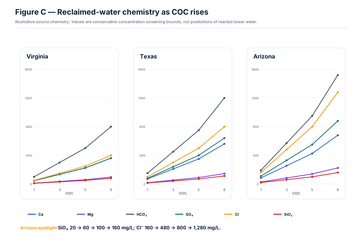
Figure C — Conservative concentration screening. The Arizona case makes the silica/chloride ceiling visible long before COC becomes a purely hydraulic question.

Three 300 MW case studies

Water-balance results

Using the evaporation model and the COC equations above produces the following annual flows:

Site	COC	Evaporation GL/y	Blowdown GL/y	Makeup GL/y	Average makeup MGD
Virginia	3	2.570	1.285	3.854	2.790
Virginia	5	2.570	0.642	3.212	2.325
Virginia	8	2.570	0.367	2.937	2.125
Texas	3	3.212	1.606	4.818	3.487
Texas	5	3.212	0.803	4.015	2.906
Texas	8	3.212	0.459	3.671	2.657
Arizona	3	3.854	1.927	5.782	4.184
Arizona	5	3.854	0.964	4.818	3.487
Arizona	8	3.854	0.551	4.405	3.188

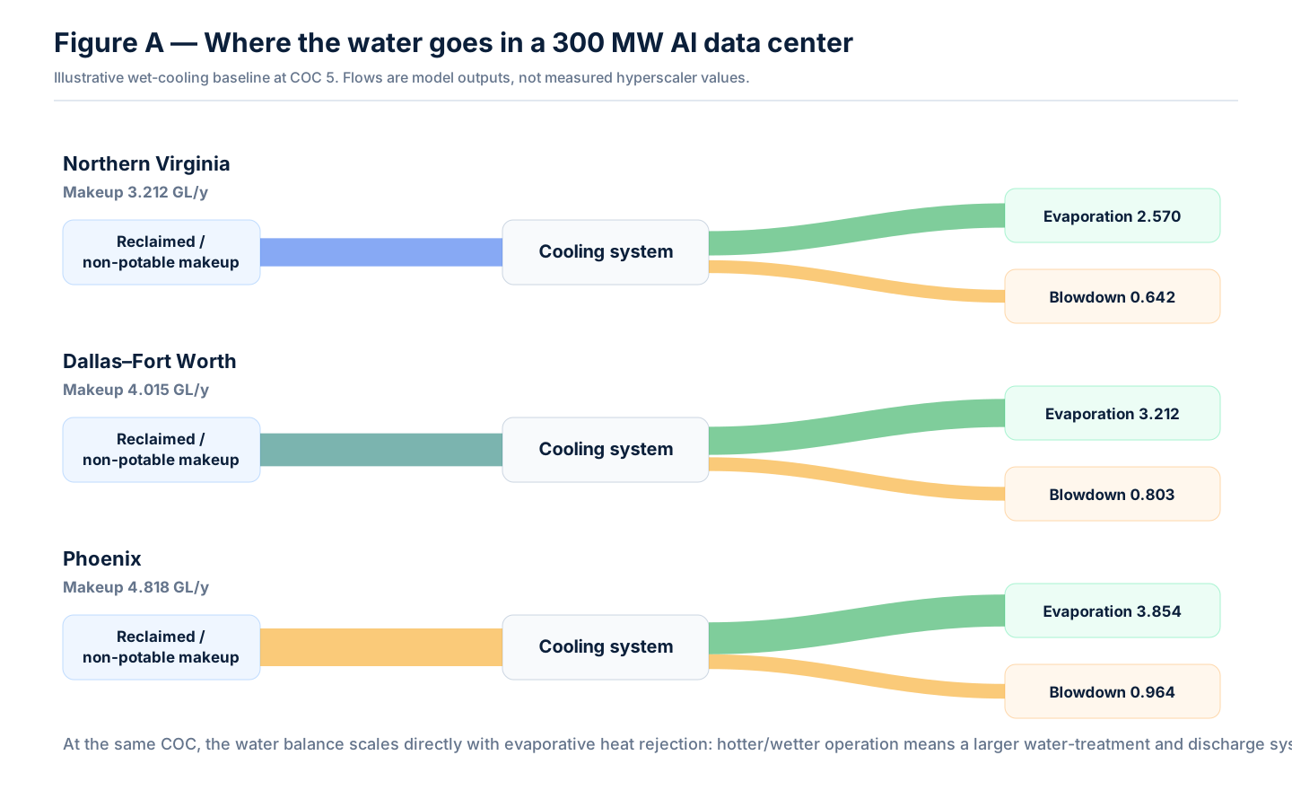
Figure A — At the same COC, water-system scale is primarily set by how much heat still reaches evaporative rejection.

The hydraulic lesson is straightforward. A 300 MW campus with a large wet-heat fraction is not a small industrial-water customer. Even when COC is pushed to 5, the modeled makeup demand ranges from about 3.2 to 4.8 GL/y across the three cases. The chemistry lesson is less obvious: the site with the greatest water savings incentive is often also the site where pushing COC is chemically hardest.

Northern Virginia: reclaimed-water infrastructure is the structural advantage

For the illustrative Virginia reclaimed makeup, conservative concentration gives:

Parameter, mg/L	Makeup	COC 3	COC 5	COC 8
Ca	45	135	225	360
Mg	12	36	60	96
HCO₃	100	300	500	800
SO₄	45	135	225	360
Cl	50	150	250	400
SiO₂	10	30	50	80
TOC	4	12	20	32
NH₄-N	0.5	1.5	2.5	4.0

At COC 5 the theoretical chloride concentration reaches about 250 mg/L; at COC 8 it reaches about 400 mg/L. These values are not universal corrosion thresholds. Materials, temperature, pH and the inhibitor program still govern actual risk. But they are enough to show why COC 8 cannot be selected by conductivity alone.

Virginia’s real advantage is not just climate. Loudoun already has a reclaimed-water network and a high-grade treatment plant. That creates a plausible design route in which reclaimed water + moderate COC + hybrid dry/wet heat rejection can be evaluated before a full-flow membrane plant is assumed.

A reasonable first-pass train is:

$$\text{Reclaimed water} \rightarrow \text{filtration as required} \rightarrow \text{selective softening} \rightarrow \text{chemical conditioning} \rightarrow \text{cooling system}$$

with COC 4–6 as an initial pilot/optimization range rather than a guaranteed operating target.

Texas: water quantity and chemistry both become first-order constraints

For the illustrative Texas reclaimed case:

Parameter, mg/L	Makeup	COC 3	COC 5	COC 8
Ca	70	210	350	560
Mg	18	54	90	144
HCO₃	150	450	750	1,200
SO₄	80	240	400	640
Cl	100	300	500	800
SiO₂	14	42	70	112
TOC	6	18	30	48
NH₄-N	1.0	3	5	8

By COC 5, the water is no longer something that can be managed by a conductivity controller alone. Calcium and alkalinity both rise sharply, chloride is at 500 mg/L in the conservative screen, TOC reaches 30 mg/L, and the biological-control burden grows with warmer water. At COC 8, silica exceeds 100 mg/L in the no-reaction upper-bound calculation and chloride reaches 800 mg/L.

Three design routes deserve comparison:

1. COC 3–4 with limited pretreatment. Higher makeup and blowdown, but simpler chemistry.
2. Softening or NF + COC 5–7. Higher treatment CAPEX, but targeted removal of multivalent scale formers without automatically desalting the entire stream.
3. D2C + dry/hybrid rejection. Reduce the amount of heat that enters the open tower in the first place.

At 300 MW scale, the third route is often more structurally scalable than continuously adding water-treatment complexity simply to force COC toward 8–10.

Arizona: the clearest water–energy–chemistry paradox

The illustrative Arizona reclaimed-water case is deliberately severe enough to expose the tradeoff:

Parameter, mg/L	Makeup	COC 3	COC 5	COC 8
Ca	85	255	425	680
Mg	28	84	140	224
HCO₃	190	570	950	1,520
SO₄	110	330	550	880
Cl	160	480	800	1,280
SiO₂	20	60	100	160
TOC	7	21	35	56
NH₄-N	1.5	4.5	7.5	12

At COC 5:

$$Ca=425\ mg/L$$

Expressed approximately as CaCO₃ hardness:

$$425\times2.497\approx1{,}061\ mg/L\ as\ CaCO_3$$

while:

$$SiO_2\approx100\ mg/L$$

and:

$$Cl^-\approx800\ mg/L$$

Again, those are not automatic failure limits. They are warning signs that further COC increase must be justified by a materials-specific saturation/corrosion model and a real chemical program.

At COC 8, the screening values become:

$$SiO_2\rightarrow160\ mg/L$$ $$Cl^-\rightarrow1{,}280\ mg/L$$ $$HCO_3^-\rightarrow1{,}520\ mg/L$$

At that point, “add more antiscalant and keep increasing COC” is not a robust design philosophy.

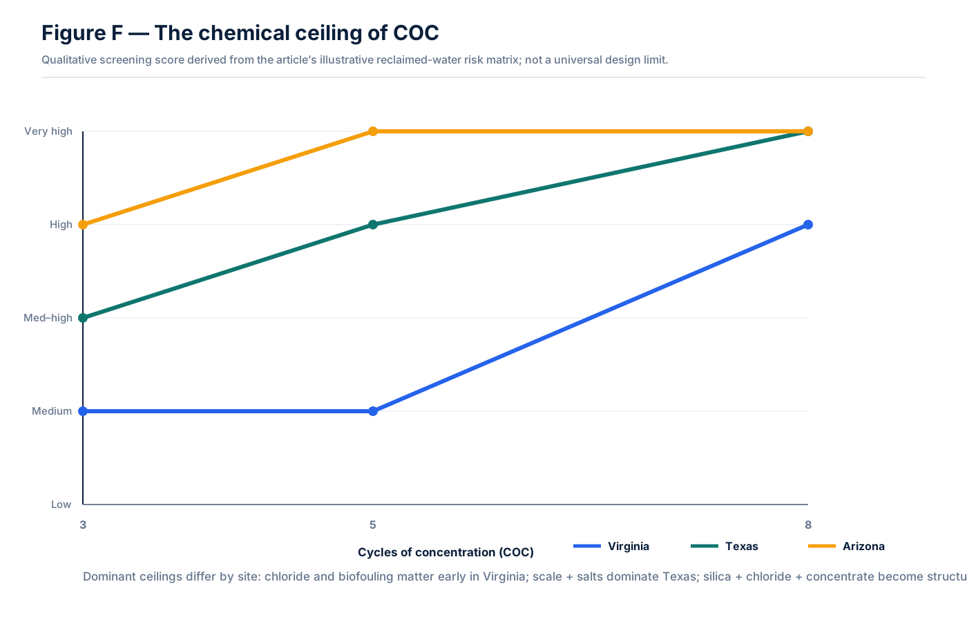
Figure F — The chemical ceiling appears at different COC values in different source-water scenarios. The chart is qualitative screening, not a universal limit.

A qualitative risk matrix makes the site differences explicit

Using the illustrative reclaimed-water chemistry, with no dedicated pretreatment, gives the following screening matrix. These ratings are not design criteria; they simply summarize where the chemistry begins to become structurally uncomfortable as COC rises.

Site	COC	Hardness / CaCO₃ scale	Silica / composite scale	Chloride / TDS corrosion	Biofouling	Overall screening risk
Virginia	3	Low–medium	Low	Medium	Medium	Medium
Virginia	5	Medium	Medium	Medium	Medium–high	Medium
Virginia	8	High	Medium–high	High	High	High
Texas	3	Medium	Medium	Medium–high	Medium–high	Medium–high
Texas	5	High	Medium–high	High	High	High
Texas	8	Very high	High	Very high	High	Very high
Arizona	3	High	Medium	High	Medium–high	High
Arizona	5	Very high	High	Very high	High	Very high
Arizona	8	Very high	Very high	Very high	Very high	Not recommended without enhanced treatment

The matrix shows why “run every tower at COC 8” is not a universal conservation strategy. Virginia has room to test moderate-to-high concentration because both climate and reclaimed-water infrastructure can reduce the hydraulic and chemistry burden. Texas reaches a multi-constraint region earlier: hardness, chloride, silica and biology all become meaningful. Arizona reaches the most severe chemistry at exactly the site where the incentive to save every unit of makeup water is strongest.

That tension is the chemical ceiling of COC. The ceiling is not the same as a theoretical solubility point. It is the practical point at which incremental water savings are no longer worth the combined cost of pretreatment, chemical control, metallurgy, cleaning frequency, reliability risk and concentrate disposal.

The three locations illustrate different kinds of scarcity

The comparison is useful because “water-stressed data center” can mean three different engineering things.

In Northern Virginia, the strategic advantage is infrastructure: dense digital development exists alongside a utility system that has already invested in high-grade reclaimed water. The principal opportunity is therefore to substitute non-potable water, preserve moderate COC, and use hybrid thermal architecture to keep both the hydraulic peak and chemistry within a manageable envelope. The limiting issue may become summer biology or chloride rather than absolute source availability.

In Texas, the problem becomes more balanced. Summer heat pushes a larger fraction of annual heat rejection toward wet operation, while the illustrative reclaimed chemistry creates simultaneous hardness, chloride, silica and biological constraints. That combination makes selective pretreatment more valuable. A project can compare the cost of additional water and blowdown at COC 3–4 against softening/NF and higher COC, while independently asking how much wet duty D2C and dry rejection can remove.

In Arizona, water scarcity and chemistry reinforce each other. The model gives the strongest incentive to reduce makeup and blowdown, yet the illustrative water also reaches the most aggressive silica and chloride levels as COC rises. This is exactly where “maximum COC” becomes a misleading conservation goal. A small reduction in wet-heat fraction can save more water than forcing the final few increments of COC, and it can do so without creating an equally difficult concentrate stream.

This is the broader lesson for siting. A site should not be ranked only by the availability of a municipal connection or reclaimed-water volume. It should be ranked by the combined ability to reject heat, supply suitable water, condition that water, discharge residuals and support the required electrical architecture under peak conditions.

The full-flow RO paradox: pretreatment can increase source-water demand

The most instructive Arizona calculation is what happens when an aggressive pretreatment is added.

At COC 8, the cooling tower requires about:

$$M_{tower,COC8}=4.405\ GL/y$$

If the entire makeup stream is produced by RO at an assumed 80% recovery:

$$R_{RO}=80\%$$

then the RO feed is:

$$Feed_{RO} = \frac{4.405}{0.80} = 5.506\ GL/y$$

and RO concentrate is:

$$5.506-4.405=1.101\ GL/y$$

while the cooling-tower blowdown itself is only:

$$0.551\ GL/y$$

So the pretreatment system creates a concentrate stream roughly twice the volume of the tower blowdown it is helping the cooling system manage.

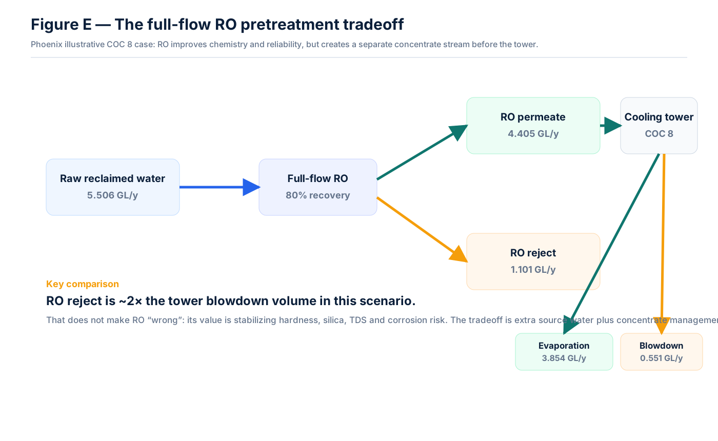
Figure E — The pretreatment tradeoff. RO may be fully justified for reliability, silica, TDS or corrosion control; the point is that its source-water and residuals penalty must be counted.

This is not an argument against RO. Commercial brackish-water RO elements can provide very high salt rejection and strong removal of silica, TOC and multivalent ions. It is an argument against assuming that “RO + high COC” automatically equals the smallest environmental footprint.

The more useful question is what chemistry actually needs to be removed. Nanofiltration can preferentially reject multivalent ions such as Ca²⁺ and Mg²⁺ while allowing more monovalent salt passage. DuPont describes NF as high-rejection for multivalent ions and lower-rejection for monovalent species. If the controlling problem is hardness rather than NaCl, selective removal can avoid over-treatment.

That is why data-center cooling is an unusually strong candidate for:

$$\boxed{\text{Partial NF/RO + bypass}}$$

If, for example, only half the makeup passes through NF and the two streams are blended:

$$C_{blend}=0.5C_{NF}+0.5C_{raw}$$

it may be possible to reduce hardness or silica enough to operate safely at COC 5–6 without paying the source-water and concentrate penalty of full-flow desalination. The site’s NF System Designer is built around exactly this type of multivalent/monovalent separation and bypass blending, while the RO System Designer can be used for recovery, permeate flow and concentrate TDS mass balance.

Partial treatment creates another optimization variable: treated fraction

Once a project abandons the assumption that 100% of the makeup must receive the same treatment, a useful new decision variable appears: the fraction of flow treated by the selective process.

Let $f$ be the fraction routed through NF or RO, with treated concentration $C_t$ and bypass concentration $C_b$. The blended makeup is:

$$C_{blend}=fC_t+(1-f)C_b$$

and the membrane feed requirement is no longer tied to the full tower makeup. If a 50% NF fraction removes most divalent hardness while allowing more monovalent salts through, it may push the calcium/sulfate scaling ceiling far enough to reach the desired COC without creating the concentrate volume of full-flow RO. The optimum fraction is therefore the smallest treated fraction that moves the controlling chemistry constraint to the required operating point.

The same idea applies to seasonal operation. A project may not need the membrane train at the same duty all year. During cool months, dry rejection can lower tower makeup and the source water may be less aggressive. During the hottest period, additional NF/RO capacity, bypass adjustment or lower COC may be used. The economic comparison should include this load profile rather than sizing every treatment process around a hypothetical constant worst case.

This is one reason water-treatment modularity is valuable in AI campuses. Thermal load, source-water chemistry and compute expansion can all change over the life of the project. A selective train with controllable bypass and staged capacity gives the operator more options than a design whose only response to changing chemistry is “increase chemical dose” or “run the entire flow through RO.”

Fit-for-purpose treatment beats “make it as pure as possible”

Cooling water is not semiconductor ultrapure water. The objective is not minimum TDS. The objective is minimum total system cost and risk at the required thermal duty:

$$\min\left[ C_{treatment} +C_{chemical} +C_{blowdown} +C_{energy} +C_{risk} \right]$$

not:

$$\min(TDS)$$

This is the fit-for-purpose philosophy behind municipal reclaimed-water reuse for industrial applications. The treatment train should remove what prevents safe operation and leave what does not need to be removed.

Technology	Primary duty	Useful feasibility starting point*	Main advantage	Main limitation / residual
Lime / chemical softening	Ca, Mg, alkalinity; some silica	Dose/pH from jar tests + saturation model	Mature at large flow; raises achievable COC	Sludge, chemical handling, multiple unit operations
Na-cycle ion exchange softening	Ca, Mg	Hardness leakage + bed capacity	Simple; no membrane reject	Regeneration brine; Na/TDS remains
UF	TSS, colloids, microbes, SDI	Membrane/vendor-specific	Stabilizes reclaimed water and protects NF/RO	Does not remove dissolved salts
NF	Ca, Mg, multivalent ions, some organics	75–90% recovery as a feasibility range, then projection/pilot	Selective softening at lower pressure than RO	Still creates concentrate; weaker Na/Cl rejection
RO	TDS, hardness, sulfate, chloride, silica, TOC	70–85% recovery as a feasibility range, then membrane projection	Strongest overall chemistry stabilization	Energy + concentrate + pretreatment requirements
GAC	TOC, micropollutants, oxidant residual	EBCT often screened around 10–20 min, then pilot	Reduces organic load and oxidant demand	Breakthrough, media replacement, possible biological growth
BAC	Biodegradable organics; some NH₄/organics	Pilot-dependent	Reduces biological nutrient load	Startup and biological control complexity
Chemical conditioning	Scale, corrosion, microbiology	No universal ppm dose	Low CAPEX and adjustable online	Chemical residuals, permit compatibility, failure sensitivity

*Ranges in this table are feasibility-screening starting points, not procurement specifications. Final values require source-water data, vendor projection and pilot/bench work where appropriate.

Three treatment archetypes follow naturally.

Low-risk potable or high-grade reclaimed water:

$$\text{Source} \rightarrow \text{side-stream filtration} \rightarrow \text{chemical conditioning} \rightarrow \text{tower}$$

Medium/high-hardness reclaimed water:

$$\text{Reclaimed} \rightarrow UF \rightarrow \text{softening or NF} \rightarrow \text{chemical conditioning} \rightarrow COC\ 5{-}7$$

High-TDS / high-silica / water-stressed site:

$$\text{Reclaimed} \rightarrow UF \rightarrow \text{partial NF/RO} \rightarrow \text{blend} \rightarrow \text{small wet trim load}$$

But for a site such as the Arizona scenario, the more powerful architecture may be:

$$\text{warm-water D2C} \rightarrow \text{dry cooler} \rightarrow \text{adiabatic trim only during extremes}$$

rather than a progressively larger full-flow water-treatment plant.

Blowdown and concentrate are siting constraints, not plumbing details

Increasing COC lowers blowdown volume while increasing its concentration. The mass balance for a component $i$ is conceptually:

$$\dot m_i = Q_M C_{M,i} - \text{precipitation/consumption}$$

Higher COC therefore produces a consistent set of tradeoffs:

• sewer hydraulic load decreases;
• salt concentration increases;
• silica/hardness precipitation risk increases;
• pretreatment becomes more demanding;
• downstream membrane recovery may become more difficult;
• ZLD or MLD feed becomes more concentrated and more scaling-prone.

A design that celebrates a small blowdown number without checking where that concentrated stream can legally and physically go is incomplete.

Residuals route	Where it can fit	Energy	CAPEX	Main advantage	Main constraint
Municipal sewer / POTW	Capacity and local limits available	Low	Low	Simplest	TDS, chloride, temperature, biocide/metal limits, utility capacity
Deep-well injection	Suitable geology and UIC permitting	Low–medium	Medium–high	Handles high salinity	Geography, permit, well integrity, long-term liability
Evaporation pond	Arid climate and land available	Low operating energy	Land/liner intensive	Simple	Footprint, seepage, wildlife/ecology, storm capacity
MLD	Water scarce but full ZLD unjustified	Medium–high	High	High recovery with small residual	Final concentrate still needs an outlet
ZLD	Liquid discharge unacceptable	High	Very high	Near-elimination of liquid discharge	Energy, scale, materials, operational complexity
Crystallization	Solid salt required	Highest	Very high	True solid/liquid terminal separation	Energy, scale, salt purity/disposal

EPA’s Underground Injection Control program makes clear that deep injection is a regulated disposal route, not a generic drain line that can be added late in design. Likewise, ZLD should not be read as “zero environmental impact.” It more accurately converts:

$$\text{liquid discharge} \rightarrow \text{electricity + chemicals + solids}$$

For projects approaching MLD/ZLD territory, this site’s Process / ZLD resource and the article Zero Liquid Discharge Is a Sequencing Problem are directly relevant because the membrane-to-thermal handoff determines much of the downstream energy and capital burden.

The architecture lock-in to avoid is obvious: build a large wet-cooling plant because water appears available; add RO because COC chemistry becomes difficult; then add ZLD because RO reject and tower blowdown cannot be discharged economically. At that point the facility may be consuming substantial electricity to manage the residuals created by a heat-rejection architecture that could have been changed earlier.

Residuals management feeds back into the water-treatment design

Discharge constraints can reverse what looks optimal on the treatment side. A high-recovery membrane system may minimize liquid volume but increase the concentration of chloride, sulfate, silica and treatment chemicals until the remaining stream no longer fits a sewer agreement. Conversely, a lower-recovery system can create a larger but less concentrated stream that may be much easier to discharge or reuse.

The same logic applies to cooling-tower blowdown. Raising COC reduces hydraulic load, which is attractive when sewer capacity is constrained. But the resulting higher salinity and inhibitor/biocide concentration may tighten the chemical permit margin. A project should therefore screen both flow-limited and concentration-limited discharge cases rather than assuming one always dominates.

Residuals also have reliability implications. If the intended outlet is a municipal sewer, a temporary restriction or capacity curtailment can force the cooling system to lower recovery or reduce wet operation. If the outlet is an evaporation pond, storm storage and liner integrity become part of data-center resilience. If the outlet is injection, well availability and permit conditions become operational dependencies. If the outlet is ZLD, crystallizer availability, scaling and thermal energy become dependencies.

For a hyperscale campus, those are not peripheral environmental systems. They can determine whether the cooling architecture can run at full compute load during the very conditions when cooling demand is highest.

The water–energy paradox must be calculated, not argued rhetorically

Site WUE is:

$$WUE_{site} = \frac{W_{site}}{E_{IT}}$$

A broader source-water metric is:

$$WUE_{source} = \frac{ W_{site}+E_{facility}\times I_{grid,water} }{E_{IT}}$$

Consider a pure sensitivity case with two 300 MW IT designs at PUE 1.10 and 1.20. The annual facility-energy difference is:

$$2.628\times(1.20-1.10)=0.2628\ TWh$$

or:

$$262.8\ GWh/y$$

If the marginal grid water-consumption intensity were assumed to be 0.5 L/kWh, the additional upstream water footprint would be:

$$262.8\times10^6\times0.5 = 131.4\ ML/y$$

At 1 L/kWh it would be about 263 ML/y.

Those are not trivial volumes. But they can still be much smaller than the several GL/y of direct evaporation in the wet-cooling baseline. So two opposite slogans are both too simple:

• “Dry cooling only shifts water use to the power grid.”
• “Zero-site-water cooling has no water footprint.”

Both can be wrong. The answer depends on PUE delta, grid generation mix, local climate, wet-heat fraction and the source-water intensity of the electricity.

Operations and monitoring: the design has to survive variable water

A high-COC design that works only at average chemistry is not a high-COC design. It is a seasonal upset waiting to happen. The operating strategy needs enough instrumentation to distinguish a hydraulic problem from a chemical problem before the response becomes “add more chemical.”

At minimum, an open cooling-water system using reclaimed makeup should continuously or routinely track:

• makeup and circulating conductivity;
• makeup flow, blowdown flow and calculated/verified COC;
• pH and temperature at the circulating-water condition;
• oxidant residual or the control variable used by the microbiological program;
• corrosion monitoring appropriate to the metallurgy;
• turbidity or suspended-solids indicators where reclaimed-water variability is meaningful;
• periodic hardness, alkalinity, chloride, sulfate and silica;
• TOC/ammonia or surrogate indicators when biological nutrient loading is part of the risk model.

The most useful operating model is not a single conductivity setpoint. It is a hierarchy. Conductivity can define a first blowdown trigger, but chemistry-specific limits should be able to lower the COC target when source water changes. If chloride increases seasonally, a fixed conductivity setpoint may unknowingly keep the tower at a chloride concentration no longer compatible with the heat exchanger. If alkalinity drops while TDS remains similar, carbonate scaling risk can fall even though conductivity does not. If ammonia increases, the disinfectant demand can change without a dramatic conductivity signal.

This is also why a project should preserve source-water identity in its historian. A reclaimed-water system supplied by multiple plants, or a campus that can switch between potable and reclaimed makeup, should know which source is active and which chemistry envelope belongs to that source. The control system should not treat every cubic meter of makeup as chemically interchangeable.

For a sophisticated campus, the COC target can therefore become dynamic rather than fixed:

$$COC_{target}=f(\text{source chemistry},\ temperature,\ metallurgy,\ treatment state,\ permit margin)$$

The concept does not require an opaque AI controller. It requires a clear set of chemistry constraints, validated sensors and a supervisory layer that is allowed to choose a safer concentration target when conditions deteriorate. The same philosophy appears throughout industrial water treatment: control the actual limiting state variable, not the easiest signal to measure.

Finally, the tower and the pretreatment plant should share alarms. A softener breakthrough, NF bypass valve failure, RO recovery shift or UF integrity problem changes the allowable tower chemistry. Conversely, a tower blowdown restriction can change the recovery target of an upstream membrane system. Treating those systems as independent skids creates exactly the kind of architecture mismatch that a hyperscale facility cannot afford.

A decision framework for a real data-center site

A data-center water study should not begin by sizing the water plant. It should proceed in this order.

1. Determine how much IT heat genuinely needs evaporative rejection

Model direct-to-chip supply/return temperature, dry-bulb and wet-bulb hours, dry-cooler approach, adiabatic trim, chiller availability, redundancy and heat reuse before committing to a wet-cooling fraction. ASHRAE’s 2026 framework places this decision at the architecture level, not as a late retrofit.

2. Run four models in parallel

$$Thermal\ Model$$ $$Water\ Balance$$ $$Water\ Chemistry$$ $$Residuals/Permit\ Model$$

The models must exchange variables. A higher coolant temperature changes economizer hours. That changes wet-heat fraction. Wet-heat fraction changes evaporation. Evaporation and COC set makeup and blowdown. Source chemistry and COC set treatment intensity. Treatment recovery changes source-water demand and concentrate. The discharge route may then constrain the allowable recovery or COC.

3. Characterize source water statistically, not with one average sample

At minimum, evaluate seasonal or monthly distributions of:

$$Ca,\ Mg,\ alkalinity,\ SiO_2,\ SO_4,\ Cl,\ TOC,\ NH_4,\ TSS,\ conductivity$$

and use 90th/95th-percentile chemistry for screening. Reclaimed-water plants can change process conditions; sewer inflow, salinity, nutrient load and industrial contributions can be seasonal. A source that looks easy on an annual average can control the design for several weeks each year.

4. Define material-specific chemistry limits

Do not use a single “maximum TDS” as the design ceiling. Define constraints such as:

$$SI_{CaCO_3}$$ $$SI_{CaSO_4}$$ $$[SiO_2]$$ $$[Cl^-]$$ $$pH,\ ORP$$

plus metallurgy-specific corrosion constraints, heat-exchanger surface temperature, disinfectant compatibility and deposit-monitoring limits.

5. Optimize COC rather than maximize it

A more honest objective function is:

$$\boxed{ \min J = C_{annualized} +\lambda_1W_{fresh} +\lambda_2E +\lambda_3W_{source} +\lambda_4R_{chemistry} +\lambda_5R_{permit} }$$

subject to constraints such as:

$$SI_i\le SI_{i,max}$$ $$Cl^-\le Cl^-_{material}$$ $$SiO_2\le SiO_{2,max}$$ $$Q_{discharge}\le Q_{permit}$$ $$C_{discharge,i}\le C_{permit,i}$$

This mathematical structure leads to an important practical conclusion:

The best COC is usually not the maximum COC.

6. Design residuals management before locking the water-recovery target

If sewer capacity is limited, that fact belongs in the membrane and tower optimization. If injection is not geologically or legally available, that belongs in the site screen. If ZLD is the only credible outlet, its energy and chemical demand belongs in the thermal/water decision from the beginning.

What the three scenarios imply

Design issue	Northern Virginia	Texas	Arizona
Preferred thermal architecture	D2C + hybrid dry/wet	D2C + dry/hybrid	Warm-water D2C + predominantly dry
Role of wet cooling	Can remain a larger assist system	Peak/seasonal	Prefer trim/peak duty
Makeup source	Reclaimed preferred where available	Reclaimed/alternative source preferred	Reclaimed/non-potable strongly preferred
Initial COC optimization range	4–6	4–6, then test higher after softening	Do not begin by chasing high COC
Preferred pretreatment	Filtration/softening as required	UF + softening/NF	Partial NF/RO or reduce wet load
Full-flow RO	Usually not first choice	Chemistry-dependent	Use cautiously
Blowdown strategy	Sewer/reuse may be realistic	Sewer/MLD/site-specific	MLD/pond/injection/site-specific
Largest structural risk	Biofouling + chloride at high COC	Scale + salts + summer demand	Water availability + silica + chloride + concentrate

The precise recommendations would change with actual weather and water analysis. The structural lesson does not: the driest and hottest site should not automatically respond to water scarcity by building the most complicated water plant. It may get more leverage by shrinking the wet-cooling duty itself.

A next-generation design philosophy for data-center water

The traditional sequence is often:

$$\text{Data Center} \rightarrow \text{Large Cooling Tower} \rightarrow \text{Find Water} \rightarrow \text{Treat Water} \rightarrow \text{Handle Blowdown}$$

A more robust sequence is:

$$\boxed{\text{Minimize Evaporative Heat Load First}}$$ $$\downarrow$$ $$\text{Use Lowest-Value Suitable Water}$$ $$\downarrow$$ $$\text{Treat Only What Chemistry Requires}$$ $$\downarrow$$ $$\text{Optimize COC, Don't Maximize It}$$ $$\downarrow$$ $$\text{Design Residuals Management Before Finalizing Recovery}$$

That sequence aligns with EPA’s push to expand recycled-water use for data-center cooling, ASHRAE’s warm-water liquid-cooling architecture, WRF’s fit-for-purpose reuse work and the direction hyperscale operators are taking through combinations of reclaimed water, hybrid cooling and zero-water-evaporation designs.

The media narrative is often that “AI data centers use too much water.” The engineering conclusion is more useful:

The water challenge of hyperscale AI infrastructure is not fundamentally a question of how much water a data center can obtain. It is a system-design question: how much heat should be rejected through evaporation, what quality of water should be used for that remaining load, how many times that water can safely be concentrated, and what happens to everything left behind.

That is why the next generation of data-center water treatment is unlikely to be defined simply by a larger RO plant. It will be defined by an integrated design of thermal architecture, source-water quality, selective pretreatment, dynamic COC and residuals management.

Key sources and further reading

• Lawrence Berkeley National Laboratory. United States Data Center Energy Usage Report: 2025 Update.
• Lawrence Berkeley National Laboratory. The water use of data center workloads: A review and assessment of key determinants.
• U.S. EPA. Water Reuse Action Plan 2.0, including Action 3.10 on recycled water for industrial and data-center cooling.
• ASHRAE. AI Data Center Framework — Integrated Design Principles.
• ASHRAE. AI Data Center Framework — Energy and Thermal Efficiency.
• Microsoft. Inside Microsoft’s two-decade push to cut water intensity while scaling for growth.
• Amazon. Water stewardship.
• Loudoun Water. Water Reclamation / Broad Run Water Reclamation Facility.
• U.S. Department of Energy. Cooling Water Efficiency Opportunities for Federal Data Centers.
• U.S. Department of Energy. Best Management Practice 10: Cooling Tower Management.
• CDC. Controlling Legionella in Cooling Towers.
• Water Research Foundation. Treating Municipal Reclaimed Water for Multipurpose Industrial Reuse Applications.
• Water Research Foundation. Advancing Non-Evaporative Cooling Technologies in the CII Sector.
• DuPont Water Solutions. Nanofiltration (NF) and Brackish Water Reverse Osmosis Solutions.
• U.S. EPA. General Information About Injection Wells.